Introduction
Instructor/Author: Zhenyuan Lu
Version: 1.0.1
This is the course notes for IE6600 Computation and Visualization course, which has covered the following semesters:



- Spring 23, Fall 22, Summer 22, Spring 22, Fall 21, Summer 21, Spring 21, Fall 20, Spring 20, Spring 19
Description
IE6600 covers basic of the R, and R Shiny for data preprocessing, and visualization. It introduces students to static and interactive visualization, dashboard, and platform that reveal information, patterns, interactions, and comparisons by paying attention to details such as color encoding, a shape selection, spatial layout, and annotation. Based on these fundamentals of analytical and creative thinking, the course then focuses on data visualization techniques and the use of the most current popular software tools that support data exploration, analytics-based storytelling and knowledge discovery, and decision-making in engineering, healthcare operations, manufacturing, and related applications.
Textbooks
Most of the course materials are borrowed from the following books/resources.
- R For Data Science (R4DS), Wickham, Hadley, and Garrett Grolemund
- R For Everyone (R4E), Lander, Jared P.
- R Markdown (RMD), Xie, Yihui, et al.
- Shiny tutorial, R Shiny
R-related Materials
- R Graphics Cookbook (RGC), Chang, Winston.
- Advanced R (ADR), Wickham, Hadley.
- R Packages (RPK), Wickham, Hadley.
- Text Mining with R (TM), Silge, Julia, and David Robinson.
Lectures
| Topic | Slides | Textbook/Materials |
|---|---|---|
| Basic of R | 📑 | R4E "Basics of R" |
| 📑 | R4E "Advanced Data Structure" | |
| R functions and the grammar of visualization | 📑 | R4DS Workflow |
| Wickham A layered grammar of graphics | ||
| (optional) R4E "Writing R functions" | ||
| Basic data visualization in R | 📑 | R4DS Data Visualization with ggplot2 |
| (optional) RGC"Quickly Exploring Data" | ||
| Data transformation with dplyr | 📑 | R4DS Data Transformation with dplyr |
| Data wrangling with tibbles, readr and tidyr | 📑 | R4DS Tibbles with tibble |
| R4DS Data Import with readr | ||
| R4DS Tidy Data with tidyr | ||
| (optional) Data wrangling with stringr, forcats | 📑 | (optional) R4DS"Strings with stringr", "Factors with forcats" |
| Visualizing Relational Data | 📑 | R4DS Relational Data with dplyr |
| Introduction to Shiny | 📑 | R Shiny Shiny tutorial |
| 📑 | ||
| Exploratory data analysis and more data visualization | 📑 | R4DS Exploratory Data Analysis |
Disclaimer
I am pretty sure there are some typing errors, spelling mistakes, etc. If you find any, please contact me via lu [dot] zhenyua [at] northeastern [dot] edu.
This work is licensed under a Creative Commons Attribution-ShareAlike 4.0 International License
FAQ in IE6600
The following are the solutions/answers covered most of the questions in the class:
R Markdown Issues
1. Error(s) with installation of tinytex/MikTex
If you have to use MikTex:
You can install the dev version of the R package tinytex:
devtools::install_github('yihui/tinytex')
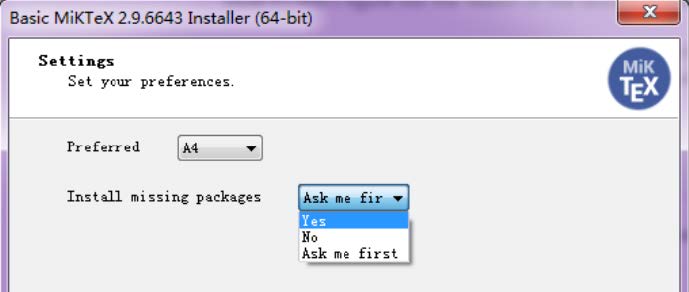
If you haven't installed MiKTeX, remember to check the option Yes in Install missing packages when installing it:
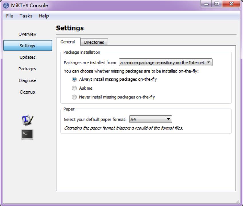
If you have already installed MiKTeX, go to the Start menu, find the menu "MiKTeX Console", and choose the option Always install missing packages on-the-fly:
If you don’t have to use MiKTeX:
Things will be a little easier. Uninstall MiKTeX if you have installed it (or temporarily rename its installation folder if you don't want to get rid of it completely), then in R:
install.packages('tinytex')
tinytex::install_tinytex()
This will install TinyTeX (a custom version of TeX Live), which can also build LaTeX documents to PDF on Windows (more info, see https://yihui.name/tinytex/). Restart RStudio/R when the installation is done (it may take 3-5 minutes).
Reference: @Yihui, https://github.com/rstudio/rmarkdown/issues/1285#issuecomment-374340175
2. If above doesn't work
If you still have issues with LaTex/tinytex, please download the following tools directly:
- For Mac user: MacTex 2022 - http://tug.org/mactex/
- For Win user: MiKTeX - https://miktex.org/download
3. If you have the pandoc error 137
Error: pandoc document conversion failed with error 137
You may have two alternative ways to deal with it (Recommended the first one):
- Knit your .rmd to .html and then print/save it as .pdf.
- Please check the post: https://stackoverflow.com/questions/51410248/r-markdown-to-html-via-knitr-pandoc-error-137?rq=1
R Language
1. Error in loading packages in Rstudio (See figure)

You have successfully loaded the ggplot2. The issue is on the package of colorspace.
Please do the following:
remove.packages(c("ggplot2", "colorspace"))
install.packages('ggplot2', dependencies = TRUE)
install.packages('colorspace', dependencies = TRUE)
2. When I use the is.character(x) or is.numeric(x) to judge the vector x, it doesn't show all result of elements.
When you assign variables into one vector, then all the elements in the vector will be treated as the same data type. But if you want to check each of the elements' data type, You may want to use the following function: sapply() or lapply()
temp<-c(1,2,"a")
sapply(temp, is.character)
3. What is coercion rule in R?
R follows the coercion rule, which means if a vector contains multiple data types it will convert a logical to a number and number to a character.
4. I can't understand the data type of factor possesses usage in R language. Could you give me some examples?
Try the following in R:
ggplot(mpg)+geom_bar(aes(drv))
ggplot(mpg)+geom_bar(aes(factor(drv, levels=c("r",4, "f"))))
5. Changing size/color by using size=0.1 or color="blue" but this kind of coding will make every point the same,
When syntax size= and color= are inside of aes()which allows you to assign variables to different sizes or colors. When they are outside of aes(), which allows you to assign constant values to size or color, 1, or "blue", etc.
R with Tableau
- How to connect R to Tableau? please check out the following tutorial on Youtube: https://www.youtube.com/watch?v=iReaNA4D2os&list=PLkqc8xRb_lIDSWEEtX9wJsngZyMPb6np3&index=7
Basic of R
Installation of R

After you click the following link: https://cran.r-project.org/
You will see as the following figure. Click the proper link and start the installation

For Mac User: Make sure you are downloading the correct version, otherwise it will cause errors
Installation of R studio
After you click the following link: https://www.rstudio.com/products/rstudio/download/
You will see as the following figure. Choose the free version, which is totally enough for our class application and practice

Tip: Update R language in Rstudio
For Windows users only:
# install package installr ----
install.pacages("installr")
# load package ----
library(installr)
# update R ----
updateR()
For Mac users:
Go to R project to download the latest R.
Note: make sure to install the correct version of R for your Mac chips.
RStudio Interface
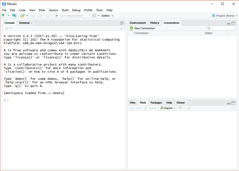
If you have successfully installed the R studio, you will see the same R studio console as the below figure showing after launching on the RStudio. (OS: Windows 10)
In this class, all the practice, homework, and project will be processing on RStudio.
R Packages
A package is essentially a library of prewritten code designed to accomplish some task or a collection of tasks. It is the most powerful tool in the R.
In this class we will be more focused on the package of ggplot2, which is most efficient package for visualization. Though there are still some very robust and well-maintained packages out there, such as dplyr, readr, caret, tibbles, or knitr.
Installation of R Packages
The fastest way to do is typing the following scripts in the Rstudio.
# install package ggplot2 (package name should be a string)
install.packages("ggplot2")
NOTE: the package name is case sensitive, which means Ggplot2 is different from ggplot2
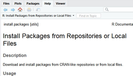
Get Help Document
There are 3 ways to get help document.
-
Press F1 (for laptop may click
Fn+F1, or "Other function key"+F1) and then the help tab will pop up on the right bottom of the RStudio. -
Type
help(install.packages) -
Type
?install.packages
Then you will see:
Un/Loading R Packages
Loading R packages (Two ways)
library(ggplot2)

Or:
require(ggplot2)

require is designed for use inside functions returning FALSE/TRUE.
Unloading R packages:
detach("package:ggplot2")
NOTE 1: You may need to load the packages again if you relaunch RStudio.
NOTE 2: It will automatedly detach all the global packages you loaded after closing Rstudio,
then follow NOTE1...

Packages Needed
You’ll also need to install some R packages. An R package is a collection of functions, data, and documentation that extends the capabilities of base R.
install.packages("tidyverse")

library(tidyverse)
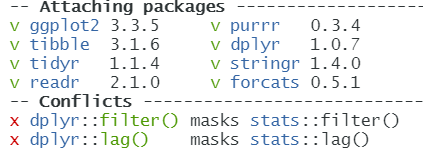
This tells you that tidyverse is loading the ggplot2, tibble, tidyr, readr,
purrr, stringr, forcats, and dplyr packages. These are considered to be the core of the tidyverse
because you’ll use them in almost every analysis.
This also tells you that there are two functions from dplyr having conflicts with stats.
You'll use dplyr:: or stats:: to specific the function from dplyr.
This is a very common issue students may have.
Installation of R Markdown
There are many other excellent packages that are not part of the tidyverse.
# install r markdown from CRAN ----
install.packages("rmarkdown")
# or if you want to test the development version ----
# install from GitHub ----
if (!requireNamespace("devtools"))
  install.packages('devtools')
devtools::install_github('rstudio/rmarkdown')
If you want to generate PDF output, you will need to install LaTeX. For R Markdown users who have not installed LaTeX before, we recommend that you install tinyteX.
# install tinyteX ----
install.packages("tinytex")

tinytex::install_tinytex()
If you have any issues with R Markdown, feel free to check: FAQ for the class
References:
[1] Hadley Wickham, Garrett Grolemund. R For Data Science.
[2] Yihui Xie, J. J. Allaire, Garrett Grolemund. R Markdown.
R Functions
Functions
R has a large collection of built-in functions that are called like this:
function_name(arg1 = val1, arg2 = val2, ...)
Let’s try using sum(), which makes regular summary of numbers. Type su and hit Tab. A pop-up shows you possible completions. Specify sum() by typing more (a “m”) to disambiguate, or by using ↑/↓ arrows to select.
sum(1,2)
## [1] 3
How to create function
The default syntax for creating a function as follow:
variable <- function(arg1, arg2,...){
  your expression/algorithm
}
Hello, World!
Now is the very cliché stuff...
If we did not include a "Hello, World!" this would not be a serious and sleepy programming class.
hello <- function(){
  print("Hello, World!")
}
hello()
## [1] "Hello, World!"
Name masking
You should have no problem predicting the output.
f <- function() {
  x <- 1
  y <- 2
  c(x, y)
}
f()
## [1] 1 2
If a name isn’t defined inside a function, R will look one level up.
x <- 2
g <- function() {
  y <- 1
  c(x, y)
}
g()
## [1] 2 1
Function inside another function
x <- 1
h <- function() {
  y <- 2
  i <- function() {
    z <- 3
    c(x, y, z)
  }
  i()
}
h()
## [1] 1 2 3
Functios created by other function
j <- function(x) {
  y <- 2
  function() {
    c(x, y)
  }
}
k <- j(1)
k()
## [1] 1 2
Functions vs Variables
The same principles apply regardless of the type of associated value — finding functions works exactly the same way as finding variables:
l <- function(x)
  x + 1
m <- function() {
  l <- function(x)
    x * 2
  l(10)
}
m()
## [1] 20
If you are using a name in a context where it’s obvious that you want a function (e.g.,f(3)), R will ignore objects that are not functions while it is searching.
n <- function(x)
  x / 2
o <- function() {
  n <- 10
  n(n)
}
o()
## [1] 5
Exercise
What does the following function return? Make a prediction before running the code yourself.
f <- function(x) {
 f <- function(x) {
   f <- function(x) {
     x ^ 2
   }
   f(x) + 1
 }
 f(x) * 2
}
f(10)
Answer:
## [1] 202
Every operation is a function call
“To understand computations in R, two slogans are helpful:
- Everything that exists is an object.
- Everything that happens is a function call.”
- John Chambers
Say a + operation between variable x and y, we can do this:
x <- 1
y <- 2
x+y
## [1] 3
Then if we set the + operator into a regular funciton format:
`+`(x,y)
## [1] 3
Another example of for
for (i in 1:2) print(i)
## [1] 1
## [1] 2
Then again for as a regular funciton:
`for`(i, 1:2, print(i))
## [1] 1
## [1] 2
Anonymous functions
Anonymouse functions shows you a side of functions that you might not have known about: you can use functions without giving them a name.
In R, functions are objects. They aren’t automatically bound to a name. Unlike other languages (e.g., Python), R doesn’t have a special syntax for creating a named function.
Generally, you use the regular assignment operator to give it a name when you create a function in R. If you choose not to give the function a name, you get an anonymous function.
The following code chunk does not call the function, but it only return the function itself.
function(x)3()
function(x)3()
You can call an anonymous function without giving it a name. You have to use the parenthesis in two ways: first, to call a function, and second to make it clear that you want to call the anonymous function itself, as opposed to calling a (possibly invalid) function inside the anonymous function:
With appropriate parenthesis, the function is called:
(function(x) 3)()
## [1] 3
Return Values
Functions are generally used for computing some value, so they need a mechanism to supply that value back to the caller.
# first build it without an explicit return
double.num <- function(x) {
  x * 2
}
double.num(5)
## [1] 10
# now build it with an explicit return
double.num <- function(x) {
  return(x * 2)
}
double.num(5)
## [1] 10
double.num <- function(x) {
  x * 3
  print("hello")
  x * 2
}
double.num(5)
## [1] "hello"
## [1] 10
double.num <- function(x) {
  return(x * 2)
  print("hello")
  return(3)
}
double.num(5)
## [1] 10
Control Statments
Control statements allow us to control the flow of our programming and cause different
things to happen, depending on the values of tests. The main control statements are
if , else, ifelse and switch.
Create one function with if and else
Let's try to create a function to demonstrate if the variable is equal to 1
if.one <- function(x){
  if(x==1){
    print("True")
  }else{
    print("False")
  }
}
if.one(1)
if.one(2)
## [1] "True"
## [1] "False"
Create one function with ifelse
Let's try to create a function to demonstrate if the variable is equal to 1
if.one <- function(x){
  ifelse(x==1, "TRUE","FALSE")
}
if.one(1)
if.one(2)
## [1] "TRUE"
## [1] "FALSE"
Create one function with switch
If we have multiple cases to check, writing else if repeatedly can be cumbersome and inefficient. This is where switch is most useful.
multipleCases <- function(x){
  switch(x,
        a="first",
        b="second",
        z="last",
        c="third",
        d="other")
}

multipleCases("a")
Special argument ...
There is a special argument called ... . This argument will match any arguments not otherwise matched, and can be easily passed on to other functions.
Example 1
f <- function(a,b,c) {
  data.frame(a,b,c)
}
f(a = 1, b = 2, c = 3)
##   a b c
## 1 1 2 3
Example 2
f <- function(...) {
  data.frame(...)
}
f(a = 1, b = 2, c = 3, d = 5, e = 7)
##   a b c d e
## 1 1 2 3 5 7
Tips
Try press Alt-Shift-K to see the shortcuts in R Studio.
for Loops
The most commonly used loop is the for loop.
for(i in 1:3){
  print(i)
}
## [1] 1
## [1] 2
## [1] 3
Let's build up a automatic for loop to count the number of letters for fruit names.
# build a vector holding fruit names
fruit <- c("apple", "banana", "pomegranate")
# make a variable to hold their lengths, with all NA to start
fruitLength <- rep(NA, length(fruit))
fruitLength
## [1] NA NA NA
# give it names
names(fruitLength) <- fruit
fruitLength
##       apple      banana pomegranate
##          NA          NA          NA
for (i in fruit){
  fruitLength[i] <- nchar(i)
}
fruitLength
##       apple      banana pomegranate
##           5           6          11
Apply Family
Built into R is the apply function and all of its common relatives such as lapply, sapply and mapply. Each has its quirks and necessities and is best used in different situations.
apply
theMatrix <- matrix(1:9, nrow=3)
# sum the rows
apply(theMatrix, 1, sum)
## [1] 12 15 18
# sum the columns
apply(theMatrix, 2, sum)
## [1] 6 15 24
Notice that this could alternatively be accomplished using the built-in rowSums and colSums functions, yielding the same results.
Sum up the row values.
rowSums(theMatrix)
## [1] 12 15 18
Sum up the column values.
colSums(theMatrix)
## [1] 6 15 24
lapply and sapply
Basic grammar:
lapply(x, FUN, ...)
sapply(x, FUN, ...)
lapply
lapply works by applying a function to each element of a list and returning the results as a list.
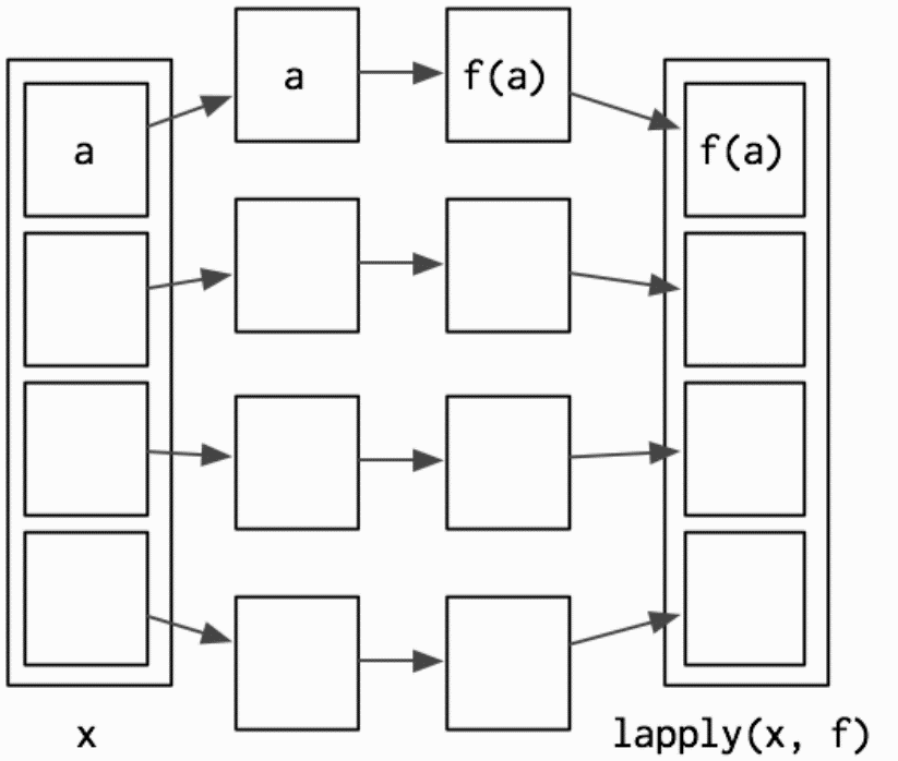
Hadley Wickham, Advanced R
lapply works by applying a function to each element of a list and returning the results as a list.
theList <- list(A=1:3, B=1:5, C=-1:1, D=2)
lapply(theList, sum)
## $A
## [1] 6
##
## $B
## [1] 15
##
## $C
## [1] 0
##
## $D
## [1] 2
sapply
sapply is a user-friendly version and wrapper of lapply by default returning a vector.
theList <- list(A=1:3, B=1:5, C=-1:1, D=2)
sapply(theList, sum)
##  A  B  C  D
##  6 15  0  2
mapply
Perhaps the most-overlooked-when-so-useful member of the apply family is mapply, which applies a function to each element of multiple lists.
firstList <-
  list(A = matrix(1:16, 4),
       B = matrix(1:16, 2),
       C = data.frame(1:5))
secondList <-
  list(A = matrix(1:16, 4),
       B = matrix(1:16, 8),
       C = data.frame(15:1))
# test element-by-element if they are identical
mapply(identical, firstList, secondList)
##     A     B     C
##  TRUE FALSE FALSE
Lets create one small function with mapply:
simpleFunc <- function(x, y) {
  nrow(x) + nrow(y)
}
mapply(simpleFunc, firstList, secondList)
##  A  B  C
##  8 10 20
References:
[1] Hadley Wickham, Advanced R
[2] Hadley Wickham, Garrett Grolemund. R For Data Science.
[3] Yihui Xie, J. J. Allaire, Garrett Grolemund. R Markdown.
[4] Jared P. Lander, Writing R functions. (NEU library)
The Grammar of Graphics
Common plots
Common statistical plots:
- Bar chart
- Scatter plot
- Line chart
- Box plot
- Histogram
The followings are the general rules for common plots, but theses can always be changed:
Scatter plot
- continuous varialbe vs continuous variable
Line plot
- continuous varialbe vs continuous variable
Box plot
- categorical varialbe vs continuous variable
Histogram
- continuous variable vs continuous variable
Bar chart
- categorical varialbe vs continuous variable
What make a basic plot
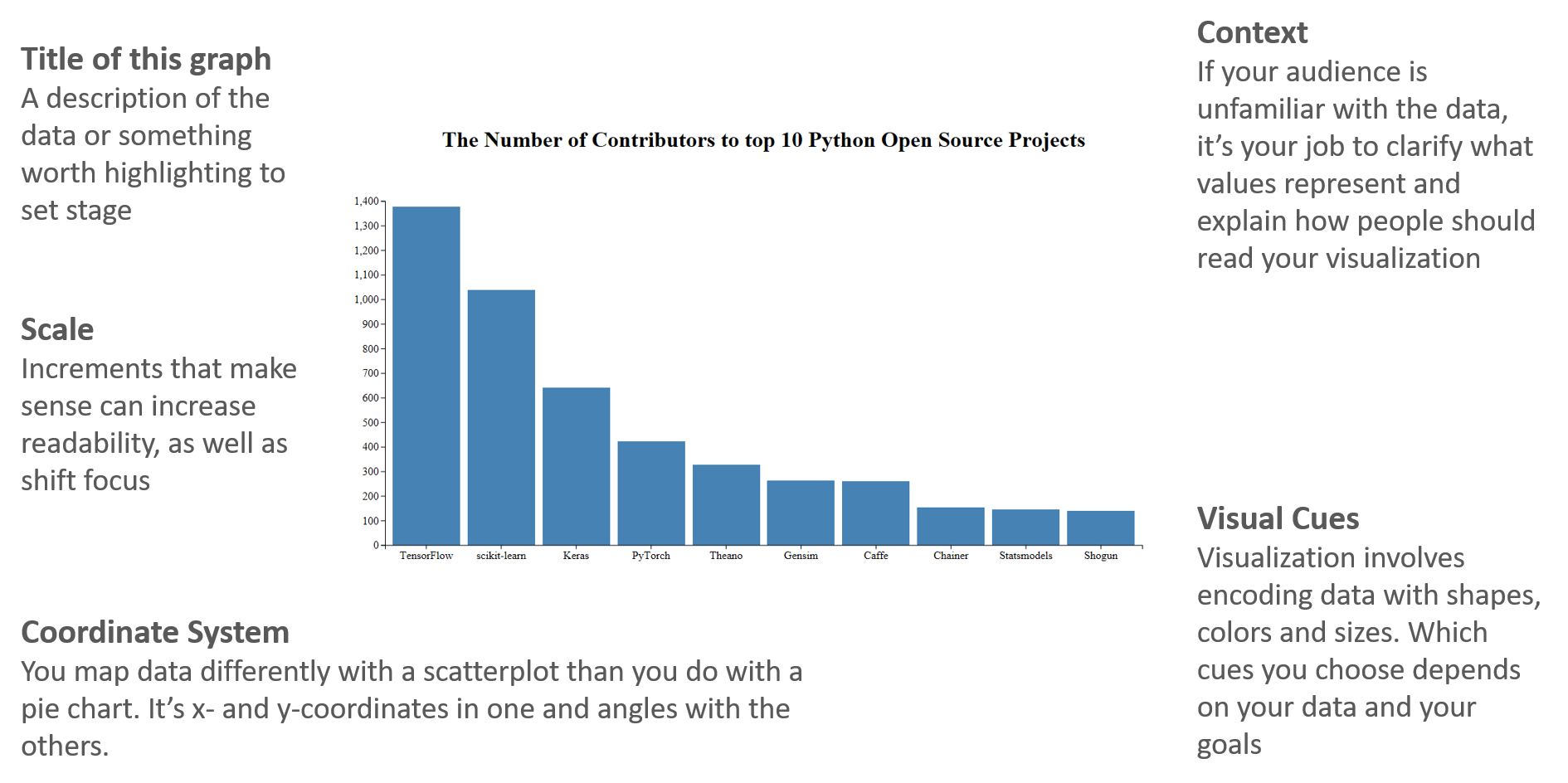
The components for a basic plot.
Let's draw a scatterplot of A vs C.
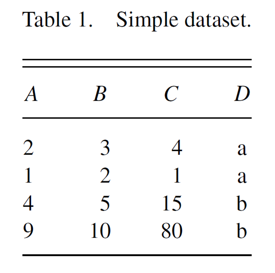
Wickham, Hadley. A Layered Grammar of Graphics.
Then Mapping A to x-position, C to y-position, and D to shape
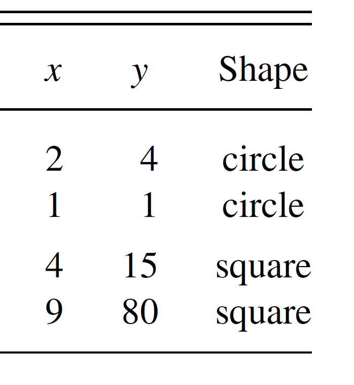
Wickham, Hadley. A Layered Grammar of Graphics.
Here we have three basic layers:
- Geometric objects
- Scales
- Coordinate system (From left to right)
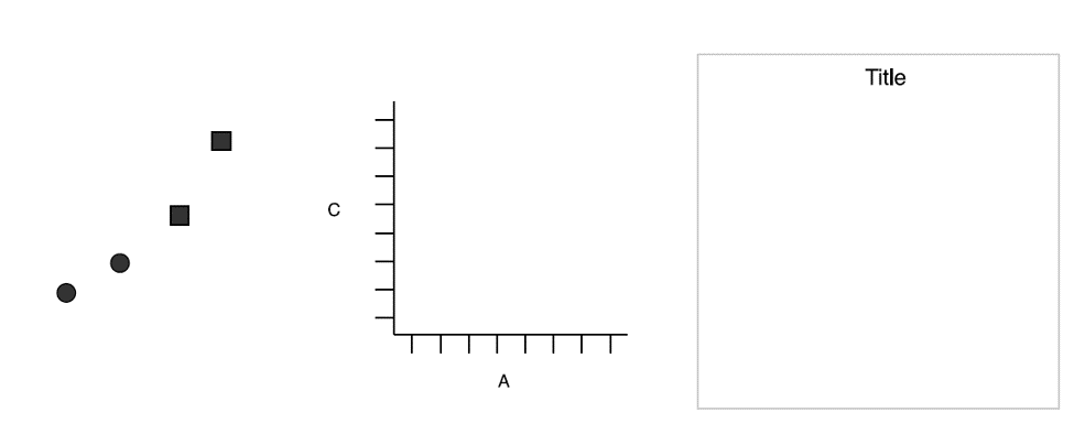
Three basic layers. Wickham.
Then we have one:
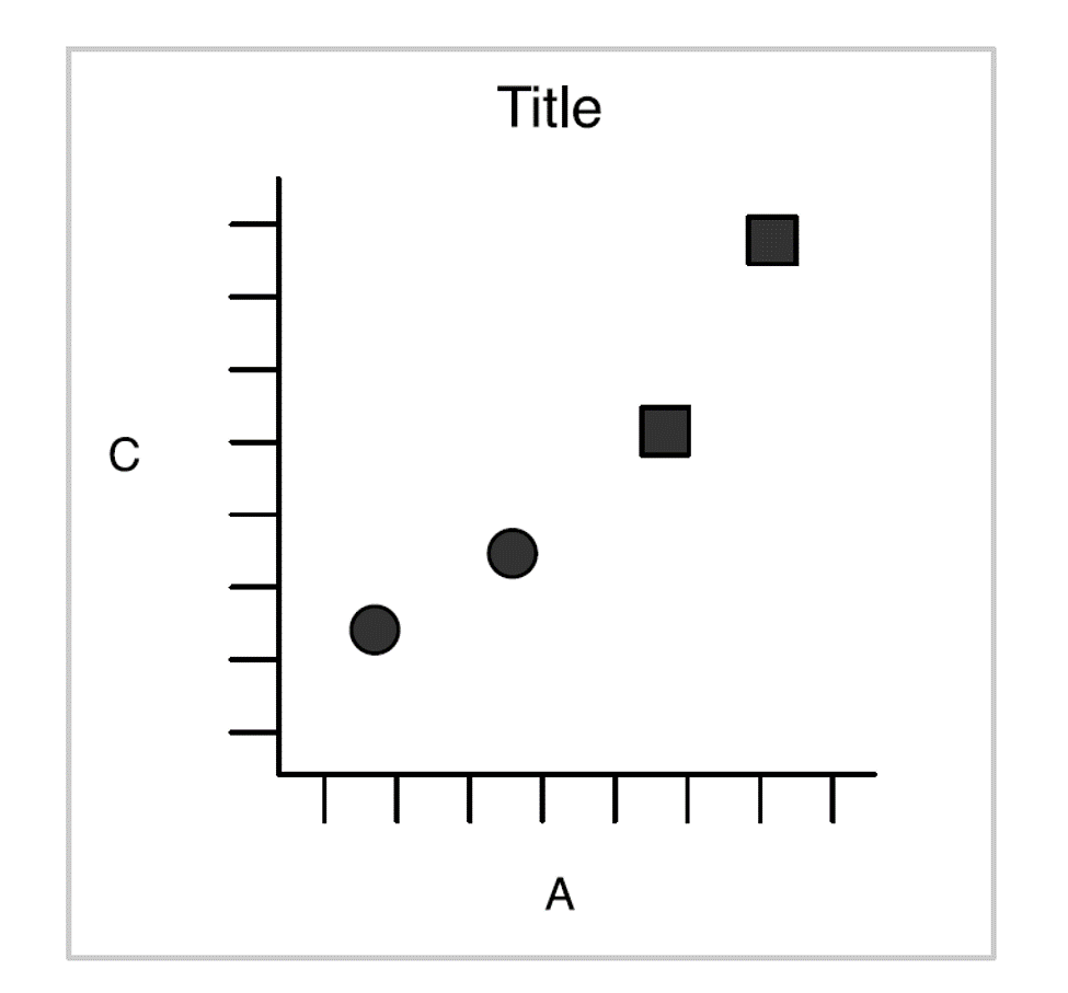
Wickham 2010
Of course, we can also create a plot by faceting:
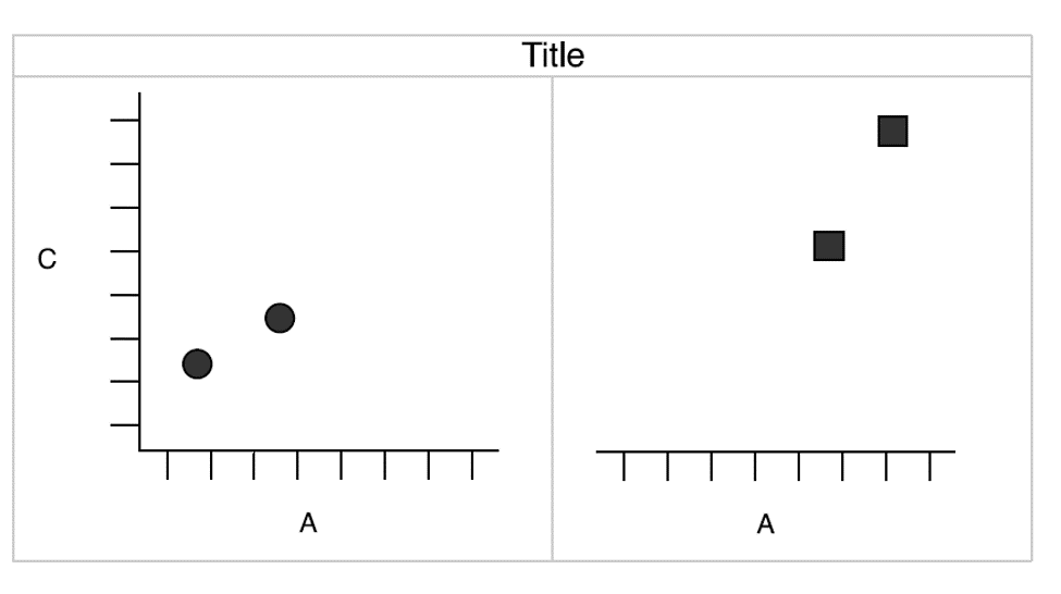
Wickham 2010
Components of the plots
- Layers:
- Dataset
- Aesthetic mapping (color, shape, size, etc.)
- Statistical transformation
- Geometric object (line, bar, dots, etc.)
- Position adjustment
- Scale (optional)
- Coordinate system
- Faceting (optional)
- Defaults
ggplot2 full syntax
ggplot2 full syntax actually is following up the above layered grammar.
ggplot(data = <DATASET>,
       mapping = aes( <MAPPINGS>) +
        layer(geom = <GEOM>,
              stat = <STAT>,
              position = <POSITION>) +
        <SCALE_FUNCTION>() +
        <COORDINATE_FUNCTION>() +
        <FACET_FUNCTION>()
Previous example
Let's get back to the previous example.
df <- data.frame(
  A = c(2, 1, 4, 9),
  B = c(3, 2, 5, 10),
  C = c(4, 1, 15, 80),
  D = c("a", "a", "b", "b")
)
df
##   A  B  C D
## 1 2  3  4 a
## 2 1  2  1 a
## 3 4  5 15 b
## 4 9 10 80 b
Questions?
- What kind of layers?
- Dataset?
- Aesthetic mapping?
- Statistical transformation?
- Geometric object?
- Position adjustment?
- Scale?
- Coordinate system?
- Faceting?
Let's make a simple ggplot2 plot based on the previous example.
ggplot(data = df,
       mapping = aes(x = A, y = C, shape = D)) +
  layer(geom = "point",
        stat = "identity",
        position = "identity") +
  scale_x_continuous() +
  scale_y_continuous() +
  coord_cartesian() +
  facet_null()
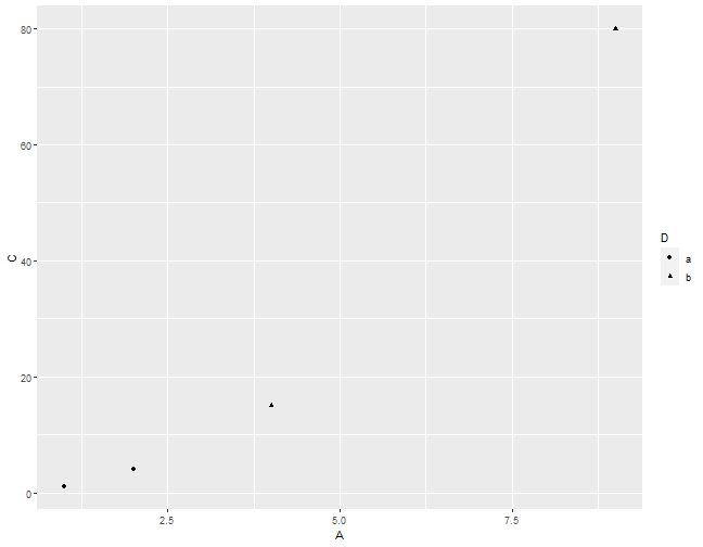
I know it's a little off from the previous example. We will cover how to adjust the background, dot size, font, etc. in the rest of the semester.

Previous example.
Facetting with grid
ggplot(data = df,
       mapping = aes(x = A, y = C, shape = D)) +
  layer(geom = "point",
        stat = "identity",
        position = "identity") +
  scale_x_continuous() +
  scale_y_continuous() +
  coord_cartesian() +
  facet_grid( ~ D)
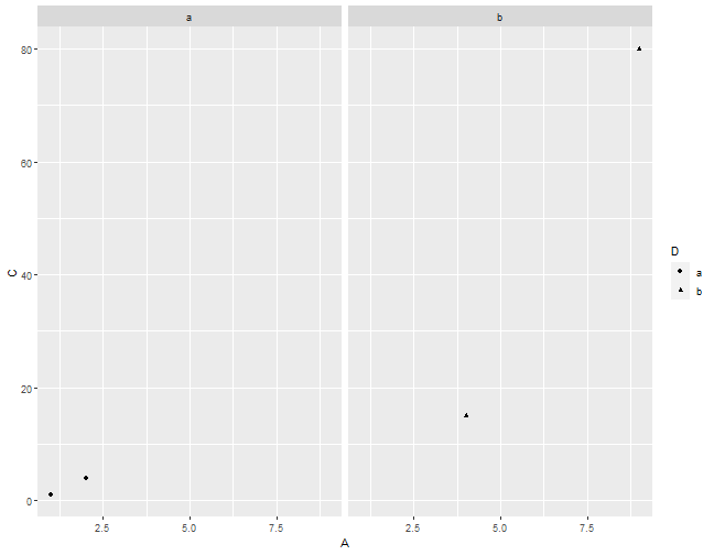
Facetting with grid.

Previous example.
A typical ggplot2
In general, we don't use full syntax of ggplot2 for our daily work.
We commonly use the following:
ggplot(data = <DATASET> ,
      mapping = aes(<MAPPINGS)) +
<GEOM_FUNCTION>()
With geom_ function
ggplot(data = df, mapping = aes(x = A, y = C, shape = D)) +
  geom_point()+
  facet_grid( ~ D)

Dataset - Fuel economy in cars
library(tidyverse)
head(mpg,5)
## # A tibble: 5 x 11
##   manufacturer model displ  year   cyl trans      drv     cty   hwy fl    class
##   <chr>        <chr> <dbl> <int> <int> <chr>      <chr> <int> <int> <chr> <chr>
## 1 audi         a4      1.8  1999     4 auto(l5)   f        18    29 p     compa~
## 2 audi         a4      1.8  1999     4 manual(m5) f        21    29 p     compa~
## 3 audi         a4      2    2008     4 manual(m6) f        20    31 p     compa~
## 4 audi         a4      2    2008     4 auto(av)   f        21    30 p     compa~
## 5 audi         a4      2.8  1999     6 auto(l5)   f        16    26 p     compa~
Dataset - Interviewing data
mpg[,c("displ","hwy")]
## # A tibble: 234 x 2
##    displ   hwy
##    <dbl> <int>
##  1   1.8    29
##  2   1.8    29
##  3   2      31
##  4   2      30
##  5   2.8    26
##  6   2.8    26
##  7   3.1    27
##  8   1.8    26
##  9   1.8    25
## 10   2      28
## # ... with 224 more rows
Dataset - Creating base
ggplot(data = mpg)

Dataset - Creating plot
ggplot(data = mpg) +
  geom_point(mapping = aes(x = displ, y = hwy))
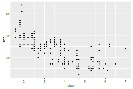
Exercise
- How many rows are in mtcars? How many columns?
- What does the drv variable describe? Read the help for ?mpg to find out.
- Make a scatterplot of hwy versus cyl.
Aesthetic mappings
We can change levels of size, shape, color, fill, alpha etc. inside of aes()
ggplot(data = mpg) +
  geom_point(mapping = aes(x = displ, y = hwy, color = class))
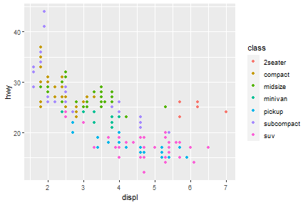
Well, if you prefer British English, you can use colour instead of color. In package of tidyverse, you may see couple of function/arguments works for either British/US English.
Aesthetic mappings - outside of aes()
You can also set the aesthetic properties of your geom manually.
ggplot(data = mpg) +
  geom_point(mapping = aes(x = displ, y = hwy), color = "red")
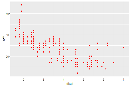
Here, the color doesn’t convey information about a variable, but only changes the appearance of the plot.
Some rules for changing the color/size/shape.
-
The name of a color as a character string
-
The size of a point in mm
-
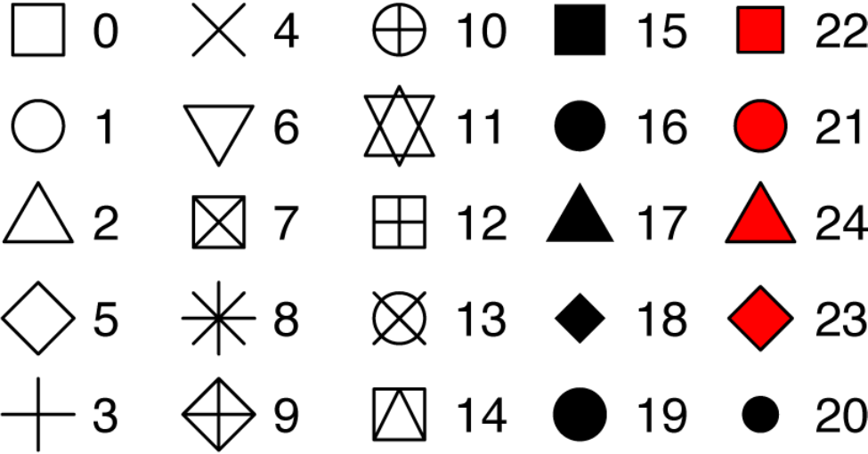
The shape of a point as a number
25 built-in shapes identified by numbers
geom_() functions
- Geometric object
- Statistical transformation
- Position adjustment
Common geom functions with geometric objects
-
geom_bar, bar chart
-
geom_histogram, histogram
-
geom_point, scatterplot
-
geom_qq, quantile-quantile plot
-
geom_boxplot, boxplot
-
geom_line, line chart
Statistical transformation
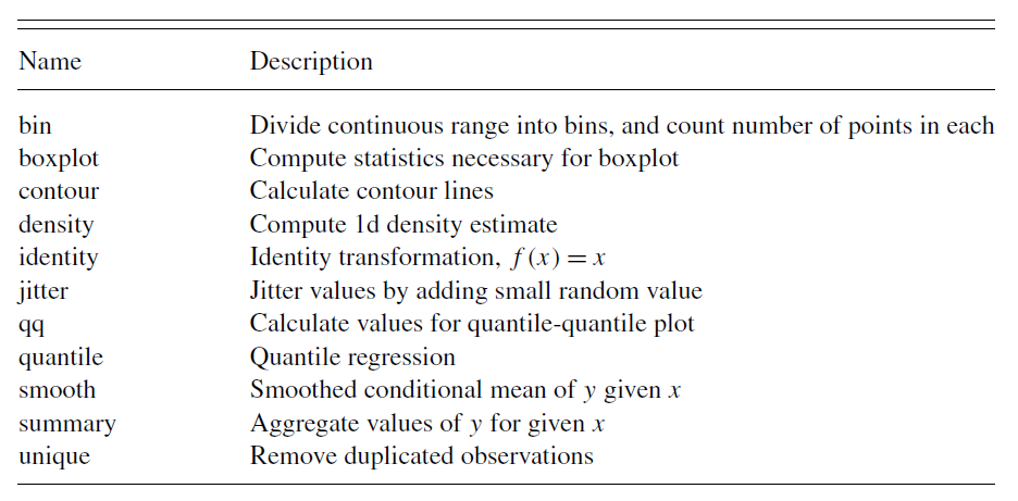
Wickham 2010.
Common geom with statistical transformation
Typically, you will create layers using a geom_ function.
- geom_bar, bar chart
- stat="count"
- geom_histogram, histogram
- stat="bin"
- geom_point, scatterplot
- stat="identity"
- geom_qq, quantile-quantile plot
- stat="qq"
- geom_boxplot, boxplot
- stat="boxplot"
- geom_line, line chart
- stat="identity"
The defaults stat and position of geom_
Check the documentation
?geom_line
Check the function
geom_line
## function (mapping = NULL, data = NULL, stat = "identity", position = "identity",
##     na.rm = FALSE, orientation = NA, show.legend = NA, inherit.aes = TRUE,
##     ...)
## {
##     layer(data = data, mapping = mapping, stat = stat, geom = GeomLine,
##         position = position, show.legend = show.legend, inherit.aes = inherit.aes,
##         params = list(na.rm = na.rm, orientation = orientation,
##             ...))
## }
## <bytecode: 0x000000001281e898>
## <environment: namespace:ggplot2>
Set of rules
- Use
geom_ functionto make variables visible on the screen. - Use
stat_ functionand define geom shape as an argument insidegeom_. - Or use
geom_and define statistical transformation as an argument inside stat_.
Common geom with position adjustments
point: geom_point, geom_jitter
Scale syntax
scale_<name>_<prepacked scale>()
Several common scale functions:
labs() xlab() ylab() ggtitle()
lims() xlim() ylim()
scale_colour_brewer()
scale_colour_continuous()
Scale example
ggplot(data = mpg) +
  geom_point(mapping = aes(x = displ, y = hwy, color=hwy))+
  scale_colour_continuous(type="viridis")
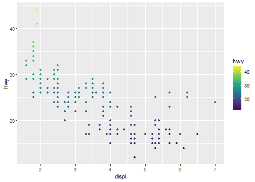
Coordinate system
ggplot(data = mpg) +
  geom_point(mapping = aes(x = displ, y = hwy))+
  coord_polar()
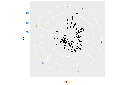
Faceting
facet_grid
ggplot(data = mpg) +
  geom_point(mapping = aes(x = displ, y = hwy))+
  facet_grid(.~year)
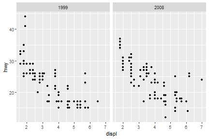
facet_wrap
ggplot(data = mpg) +
  geom_point(mapping = aes(x = displ, y = hwy))+
  facet_wrap(.~cyl)
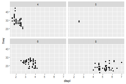
A more complicated-embedded grammar
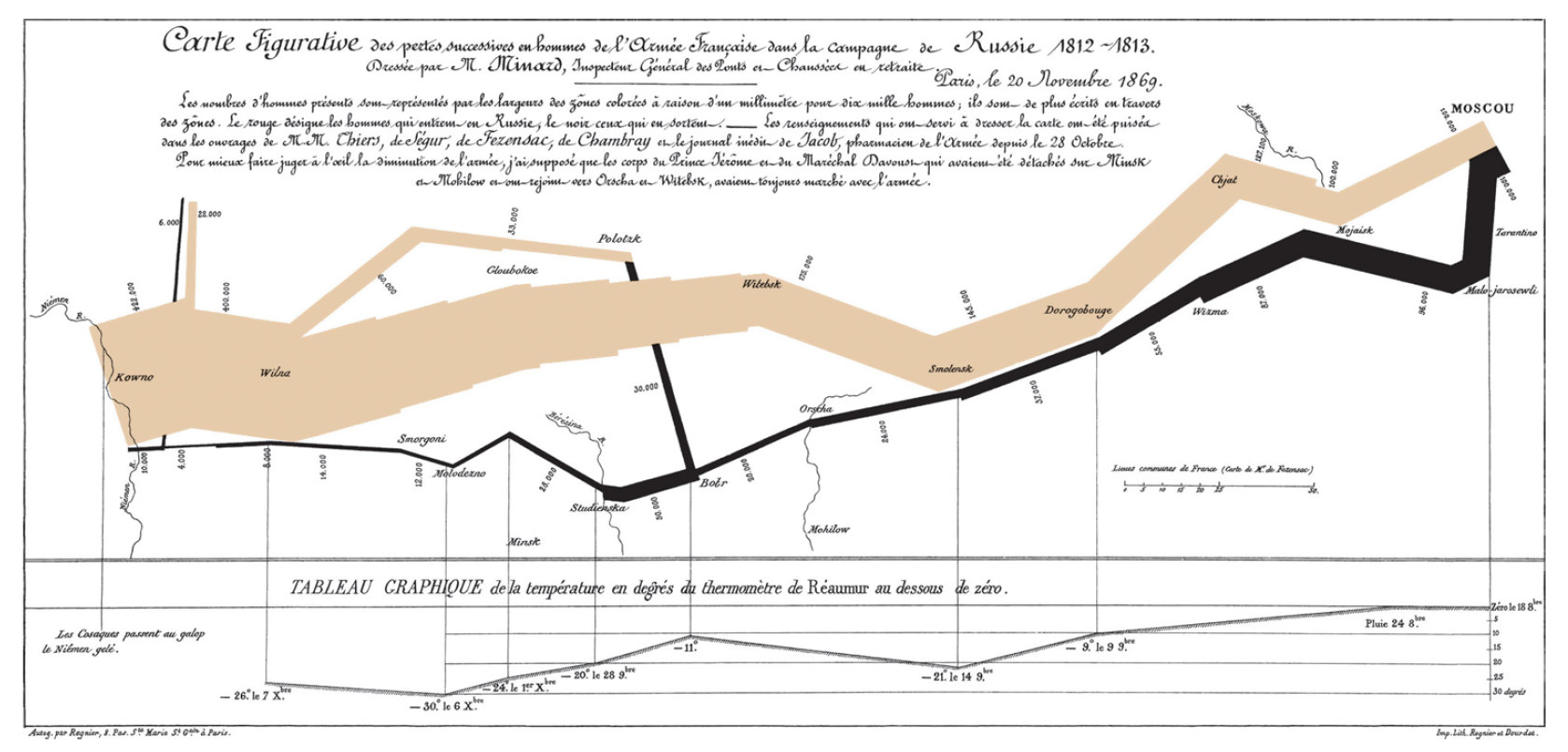
The map of Napoleon's Russian campaign
Charles Joseph Minard is best known for his cartographic depiction of numerical data on a map of Napoleon's disastrous losses suffered during the Russian campaign of 1812 (in French, Carte figurative des pertes successives en hommes de l'Armée Française dans la campagne de Russie 1812–1813). The illustration depicts Napoleon's army departing the Polish-Russian border. A thick band illustrates the size of his army at specific geographic points during their advance and retreat. It displays six types of data in two dimensions: the number of Napoleon's troops; the distance traveled; temperature; latitude and longitude; direction of travel; and location relative to specific dates without making mention of Napoleon; Minard's interest lay with the travails and sacrifices of the soldiers. This type of band graph for illustration of flows was later called a Sankey diagram, although Matthew Henry Phineas Riall Sankey used this visualisation 30 years later and only for thematic energy flow. - Wiki
Let's reproduce the top part of Minard’s famous depiction of Napoleon’s march on Russia.
This graphic can be thought of as a compound graphic:
- The top part displays the number of troops during the advance and the retreat
- The bottom part shows the temperature during the advance
We will focus on the top part of the graphic. This part displays two datasets: cities and troops. Each city has a position (a latitude and longitude) and a name, and each troop observation has a position, a direction (advance or retreat), and number of survivors.
Load data: minard-troops.txt and minard-cities.txt
Supplemental files for "A layered grammar of graphics"
- minard-cities.txt: Location of cities in Napoleon's march by Minard.
- minard-troops.txt: Troop movement data.
troops <- read.table("minard-troops.txt", header=T)
cities <- read.table("minard-cities.txt", header=T)
troops
head(troops)
##   long  lat survivors direction group
## 1 24.0 54.9    340000         A     1
## 2 24.5 55.0    340000         A     1
## 3 25.5 54.5    340000         A     1
## 4 26.0 54.7    320000         A     1
## 5 27.0 54.8    300000         A     1
## 6 28.0 54.9    280000         A     1
cities
head(cities)
##   long  lat      city
## 1 24.0 55.0     Kowno
## 2 25.3 54.7     Wilna
## 3 26.4 54.4  Smorgoni
## 4 26.8 54.3 Moiodexno
## 5 27.7 55.2 Gloubokoe
## 6 27.6 53.9     Minsk
How would we create this graphic with the layered grammar?
- Start with the essence of the graphic: a path plot of the troops data, mapping direction to color and number of survivors to size.
- Then take the position of the cities as an additional layer
- Then polish the plot by carefully tweaking the default scales
Start with the essence of the graphic: a path plot of the troops data, mapping direction to color and number of survivors to size.
plot_troops <- ggplot(troops, aes(long, lat)) +
  geom_path(aes(size = survivors, colour = direction, group = group))
plot_troops

Then take the position of the cities as an additional layer.
plot_both <- plot_troops +
  geom_text(aes(label = city), size = 4, data = cities)
plot_both

Then polish the plot by carefully tweaking the default scales.
plot_polished <- plot_both +
  scale_size(
    range = c(0, 12),
    # breaks = c(10000, 20000, 30000),
    # labels = c("10,000", "20,000", "30,000")
  ) +
  scale_color_manual(values = c("tan", "grey50")) +
  coord_map() +
  labs(title = "Map of Napoleon's Russian campaign of 1812") +
  theme_void() +
  theme(legend.position = "none")
plot_polished

I admitted that there is still huge room to improve this plot, but it gives us some taste of how to use R to mimic this classical visualization created hundred years ago by Minard.
References
[1] Hadley Wickham, Garrett Grolemund. R For Data Science.
[2] Hadley Wickham, A layered grammar of graphics
[3] ggplot2 references
Basic Data Visualization in R
Chart selection
A great explanation on selecting a right chart type by Dr. Andrew Abela.
but as a data scientist should not be limited by this.

Components of the plots
- Layers:
- Dataset
- Aesthetic mapping (color, shape, size, etc.)
- Statistical transformation
- Geometric object (line, bar, dots, etc.)
- Position adjustment
- Scale (optional)
- Coordinate system
- Faceting (optional)
- Defaults
ggplot2 full syntax
ggplot(data = <DATASET>,
       mapping = aes( <MAPPINGS>) +
        layer(geom = <GEOM>,
              stat = <STAT>,
              position = <POSITION>) +
        <SCALE_FUNCTION>() +
        <COORDINATE_FUNCTION>() +
        <FACET_FUNCTION>()
A typical graph template
ggplot(data = <DATASET> ,
      mapping = aes(<MAPPINGS)) +
      <GEOM_FUNCTION>()
Creat a plot with basic data
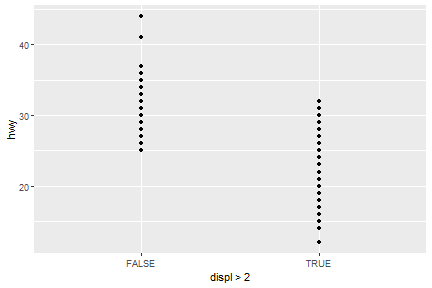
ggplot(data=mpg)+
  geom_point(mapping = aes(x=displ>2,y=hwy))
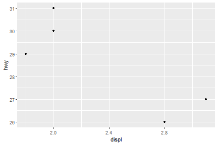
ggplot(data=mpg[mpg$model=="a4",])+
  geom_point(mapping = aes(x=displ,y=hwy))
Aesthetic Mappings
The greatest value of a picture is when it forces us to notice what we never expected to see.
—John Tukey
Basic components of aesthetic mapping:
- Mapping
- Size
- Alpha
- Shape
- Color
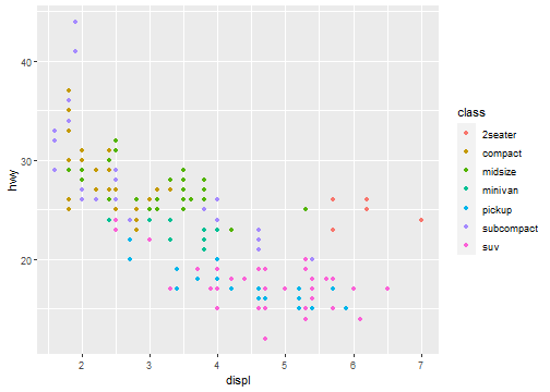
Map the colors of your points to the class variable to reveal the class of each car:
Aesthetic Mappings: Mapping
ggplot(data = mpg) +
  geom_point(mapping = aes(x = displ, y = hwy, color = class))
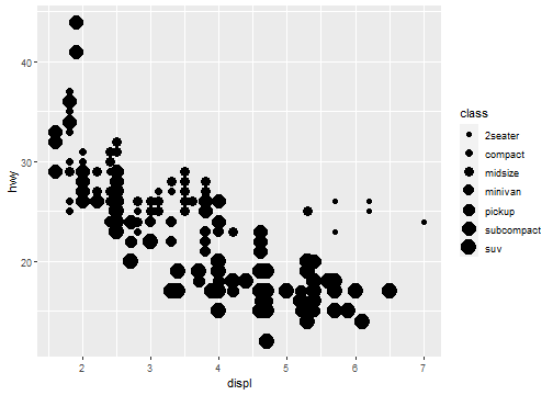
Aesthetic Mappings: Size
Not recommend mapping an unordered variable to an ordered aesthetic:
ggplot(data = mpg) +
  geom_point(mapping = aes(x = displ, y = hwy, size = class))
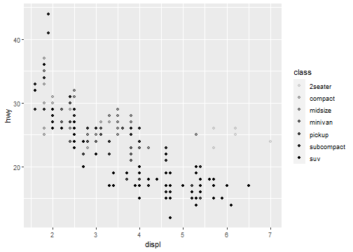
Aesthetic Mappings: Alpha
ggplot(data = mpg) +
  geom_point(mapping = aes(x = displ, y = hwy, alpha = class))
Aesthetic Mappings: Shape
ggplot(data = mpg) +
  geom_point(mapping = aes(x = displ, y = hwy, shape = class))
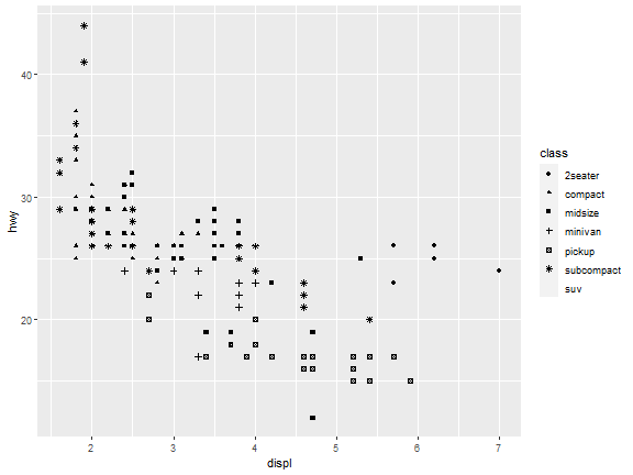
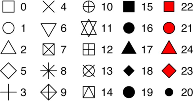
What happened to the SUVs? ggplot2 will only use six shapes at a time.
By default, additional groups will go unplotted when you use this aesthetic.
R has 25 built-in shapes that are identified by numbers
Aesthetic Mappings: Color
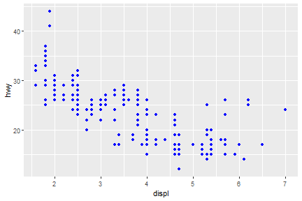
For each aesthetic you use, the aes() to associate the name of the aesthetic with a variable to display. The aes() function gathers together each of the aesthetic mappings used by a layer and passes them to the layer’s mapping argument.
ggplot(data = mpg) +
  geom_point(mapping = aes(x = displ, y = hwy), color = "blue")
Exercise
Which variables in mpg are categorical? Which variables are continuous? (Hint: type ?mpg to read the documentation for the dataset.) How can you see this information when you run mpg?
Map a continuous variable to color, size, and shape. How do these aesthetics behave differently for categorical versus continuous variables?
Facets
Facets: facet_wrap()
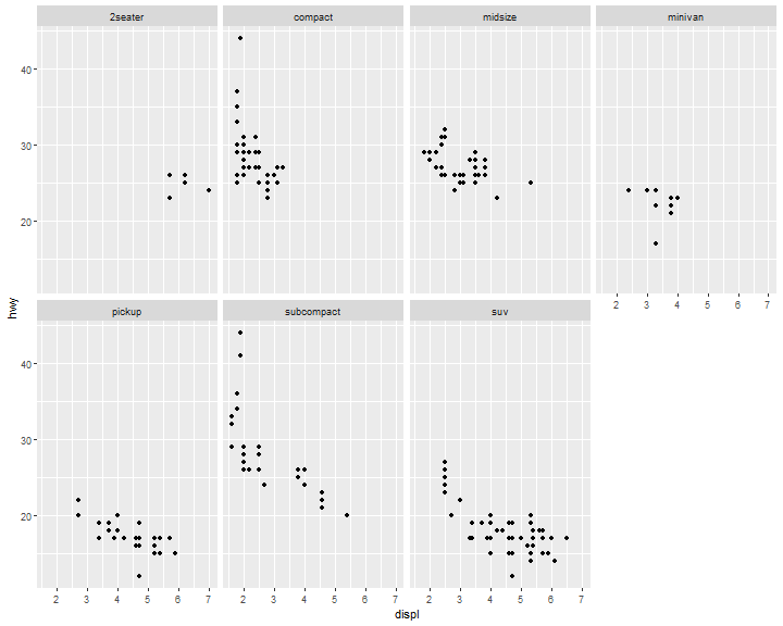
The first argument of facet_wrap() should be a formula, which you create with ~ followed by a variable name (here “formula” is the name of a data structure in R, not a synonym for “equation”). To facet your plot by a single variable (discrete), use facet_wrap()
ggplot(data = mpg) +
  geom_point(mapping = aes(x = displ, y = hwy)) +
  facet_wrap( ~ class, nrow = 2)
Facets: facet_grid()
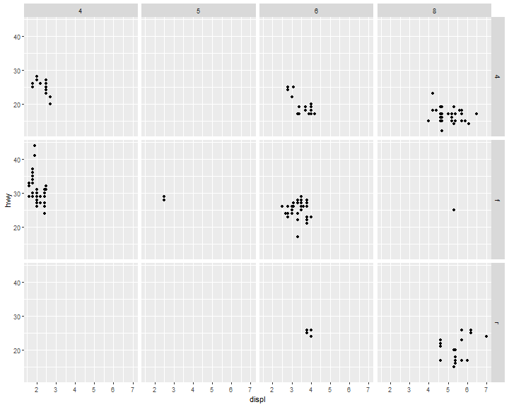
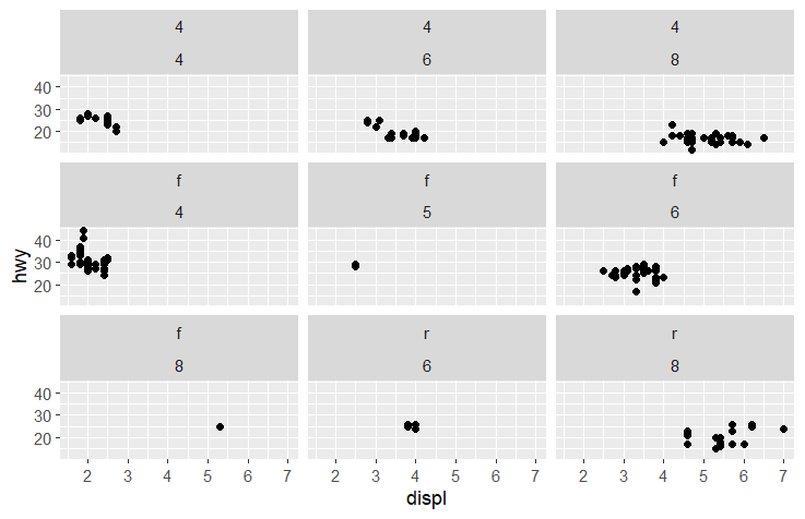
To facet your plot on the combination of two variables, add facet_grid() to your plot call.
ggplot(data = mpg) +
  geom_point(mapping = aes(x = displ, y = hwy)) +
  facet_grid(drv ~ cyl)
Tip:
If you want to use
facet_wrapto do the above plot.ggplot(data = mpg) + geom_point(mapping = aes(x = displ, y = hwy)) + facet_wrap(drv ~ cyl)You will see,
This is the difference between `facet_wrap` and `facet_grid`.
Geometric Objects
A geom is the geometrical object that a plot uses to represent data. People often describe plots by the type of geom that the plot uses. For example, bar charts use bar geoms, line charts use line geoms, boxplots use boxplot geoms, and so on.
ggplot(data = mpg) +
  geom_point(mapping = aes(x = displ, y = hwy))

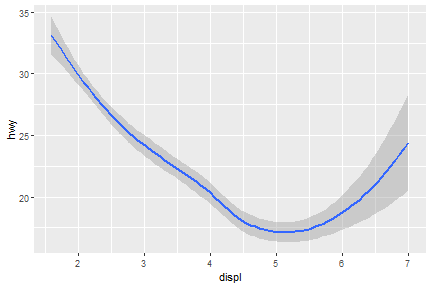
geom_smooth(): 95% confidence level interval for predictions
ggplot(data = mpg) +
  geom_smooth(mapping = aes(x = displ, y = hwy))
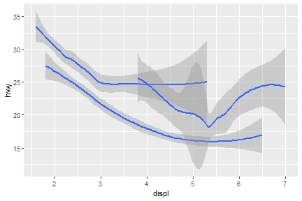
What if we would like to group the smooth_line by drv?
ggplot(data = mpg) +
  geom_smooth(mapping = aes(x = displ, y = hwy, group = drv))
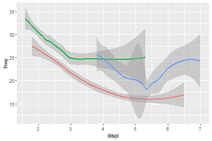
Now, arrange colors on different type of drv.
ggplot(data = mpg) +
  geom_smooth(mapping = aes(x = displ, y = hwy, color = drv),
  show.legend = FALSE)
We can also add up one more geom layer to the current one.
ggplot(data = mpg) +
  geom_point(mapping = aes(x = displ, y = hwy)) +
  geom_smooth(mapping = aes(x = displ, y = hwy))
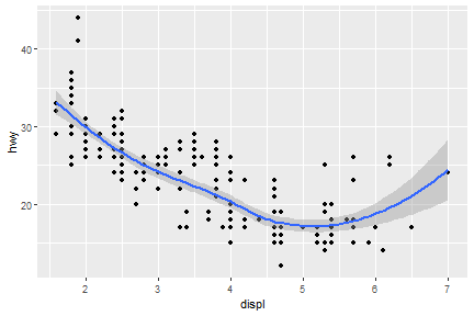
Global and local mappings
ggplot(data = mpg) +
  geom_point(mapping = aes(x = displ, y = hwy)) +
  geom_smooth(mapping = aes(x = displ, y = hwy))
ggplot2 will treat these mappings as global mappings that apply to each geom in the graph. In other words, this code will produce the same plot as the previous code:
ggplot(data = mpg, mapping = aes(x = displ, y = hwy)) +
  geom_point() +
  geom_smooth()
Local mappings
ggplot(data = mpg) +
  geom_point(mapping = aes(x = displ, y = hwy)) +
  geom_smooth(mapping = aes(x = displ, y = hwy, color=class))
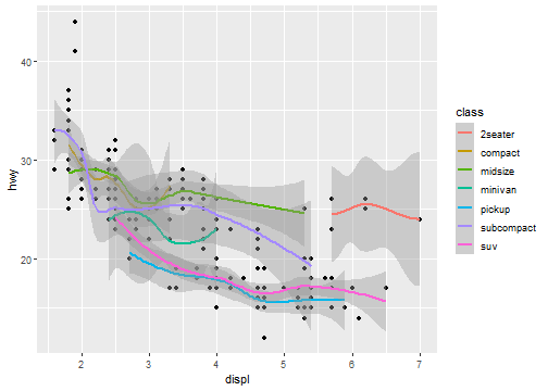
Global mapping
ggplot(data = mpg, mapping = aes(x = displ, y = hwy, color=class)) +
  geom_point() +
  geom_smooth()
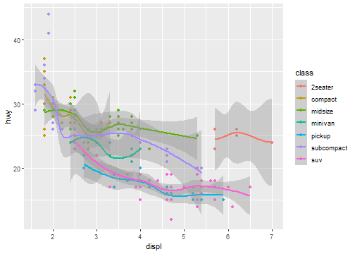
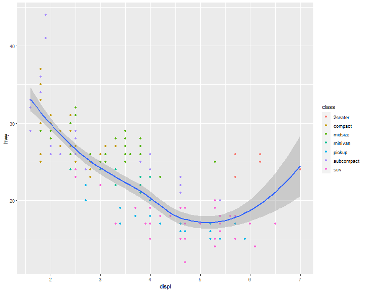
Change the color for geom_point layer only.
ggplot(data = mpg, mapping = aes(x = displ, y = hwy)) +
  geom_point(mapping = aes(color = class)) +
  geom_smooth()
Filter out data in a layer
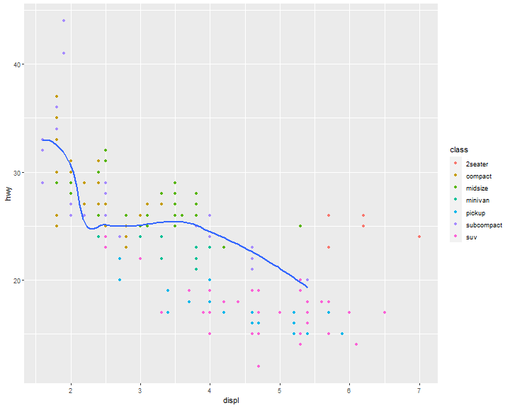
ggplot(data = mpg, mapping = aes(x = displ, y = hwy)) +
  geom_point(mapping = aes(color = class)) +
  geom_smooth(data = mpg[mpg$class == "subcompact", ],
  se = FALSE)
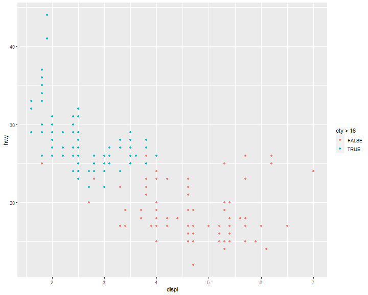
ggplot(data = mpg, mapping = aes(x = displ, y = hwy)) +
  geom_point(mapping = aes(color = cty>16))
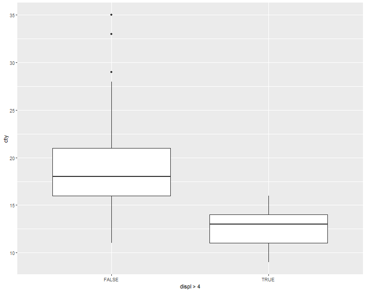
ggplot(data = mpg, mapping = aes(x = displ>4, y = cty)) +
  geom_boxplot()
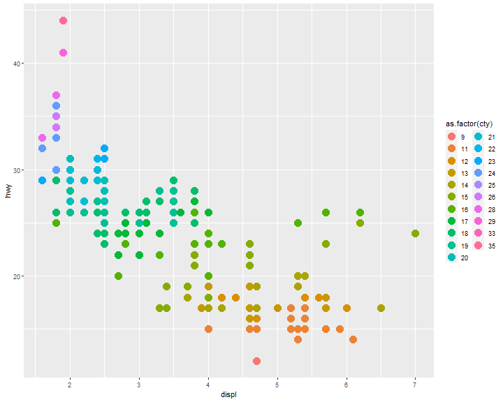
as.factor()
ggplot(mpg, aes(x = displ, y = hwy)) +
  geom_point(aes(color = as.factor(cty)), size=5)
Exercise 1
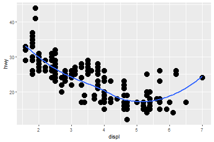
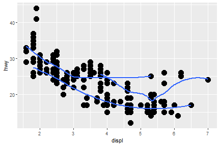
Re-create the R code necessary to generate the following graphs.
a b
a
ggplot(mpg,
       aes(x = displ, y = hwy)) +
  geom_point(size=5) +
  geom_smooth(se=F)
b
ggplot(mpg,
       aes(x = displ, y = hwy)) +
  geom_point(size=5) +
  geom_smooth(aes(class=drv),se=F)
Exercise 2
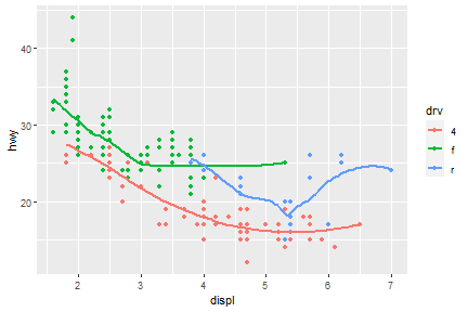
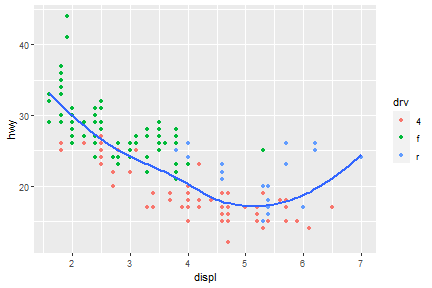
Re-create the R code necessary to generate the following graphs.
a b
a
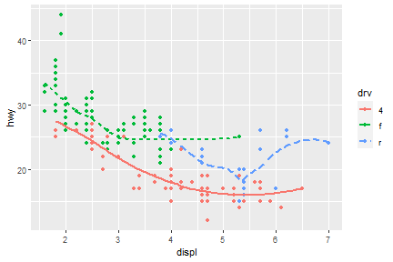
ggplot(mpg,
       aes(x = displ, y = hwy)) +
  geom_point(aes(color=drv)) +
  geom_smooth(aes(class=drv, color=drv),se=F)
b
ggplot(mpg,
       aes(x = displ, y = hwy)) +
  geom_point(aes(color=drv)) +
  geom_smooth(se=F)
Exercise 3
Re-create the R code necessary to generate the following graphs.
a b
a
ggplot(mpg,
       aes(x = displ, y = hwy)) +
  geom_point(aes(color=drv)) +
  geom_smooth(aes(class=drv, color=drv, shape=drv, linetype=drv),se=F)
b
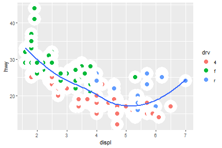
ggplot(mpg,
       aes(x = displ, y = hwy)) +
  geom_point(aes(fill=drv), shape=21, color="white", size=5, stroke=5) +
  geom_smooth(se=F)
Statistical transformation
Many graphs, like scatterplots, plot the raw values of your dataset. Other graphs, like bar charts, calculate new values to plot.
The algorithm used to calculate new values for a graph is called a stat, short for statistical transformation. The following figure describes how this process works with geom_bar().
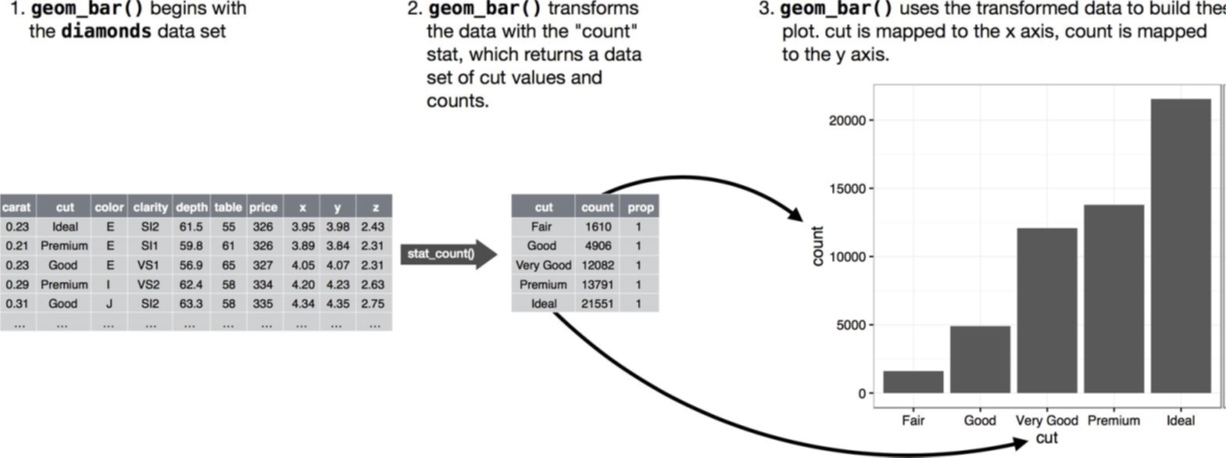
The diamonds dataset comes in ggplot2 and contains information about ~54,000 diamonds, including the price, carat, color, clarity, and cut of each diamond. The chart shows that more diamonds are available with high-quality cuts than with low quality cuts:
ggplot(data = diamonds) +
  geom_bar(mapping = aes(x = cut))

Common geom with statistical transformation
Typically, you will create layers using a geom_ function.
- geom_bar, bar chart
- stat="count"
- geom_histogram, histogram
- stat="bin"
- geom_point, scatterplot
- stat="identity"
- geom_qq, quantile-quantile plot
- stat="qq"
- geom_boxplot, boxplot
- stat="boxplot"
- geom_line, line chart
- stat="identity"
Therefore, we can use stat function instead of geom.
As we mentioned in the previous class, each stat has a default geom function.
- stat_count
- stat_qq
- stat_identity
- stat_bin
- stat_boxplot
stat_count
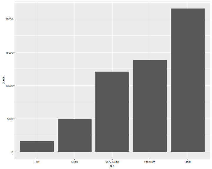
geom_bar shows the default value for stat is “count,” which means that geom_bar() uses stat_count().
geom_bar() uses stat_count() by default: it counts the number of cases at each x position.
For example, you can re-create the previous plot using stat_count() instead of geom_bar():
ggplot(data = diamonds) +
  stat_count(mapping = aes(x = cut))
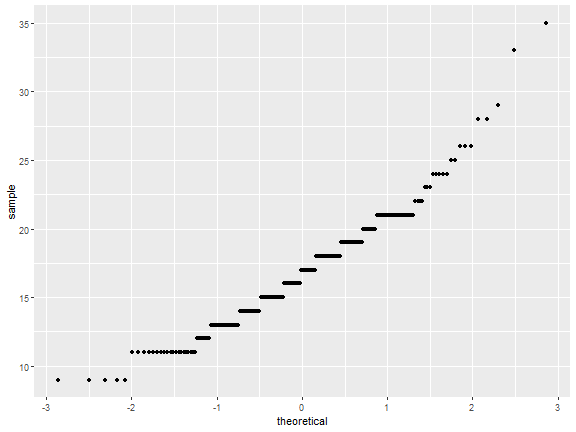
stat_qq
ggplot(mpg)+
  stat_qq(aes(sample=cty))
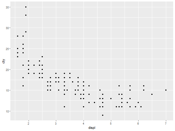
stat_identity
ggplot(mpg)+
  stat_identity(aes(displ,cty))
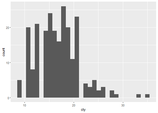
stat_bin
ggplot(mpg)+
  stat_bin(aes(cty))
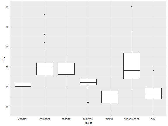
stat_boxplot
ggplot(mpg)+
  stat_boxplot(aes(class,cty))
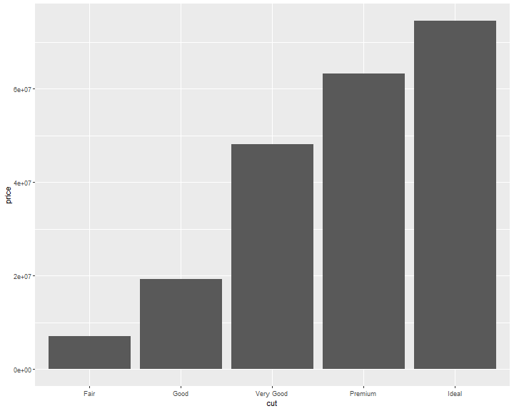
Identity stat
If you want the y axis of bar chart to represent values instead of count, use stat="identity"
ggplot(data = diamonds) +
  geom_bar(mapping = aes(x = cut, y=price), stat="identity")

If you want the heights of the bars to represent values in the data, use geom_col() instead, which is the identity stat version of geom_bar
ggplot(data = diamonds) +
  geom_col(mapping = aes(x = cut, y=price))
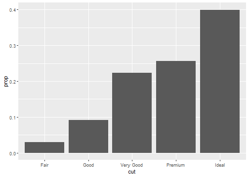
Stat proportion
ggplot(data = diamonds) +
  geom_bar(mapping = aes(x = cut, y = ..prop.., group = 1))
Position Adjustments
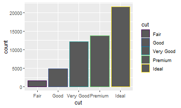
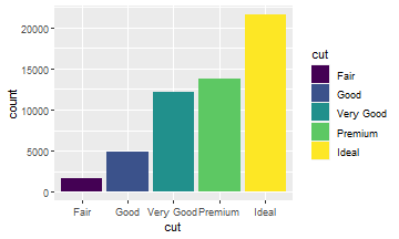
There’s one more piece of magic associated with bar charts. You can color a bar chart using either the color aesthetic, or more usefully, fill:
ggplot(data = diamonds) +
  geom_bar(aes(x = cut,
               color = cut))
ggplot(data = diamonds) +
  geom_bar(aes(x = cut,
               fill = cut))
Position Adjustments: stack
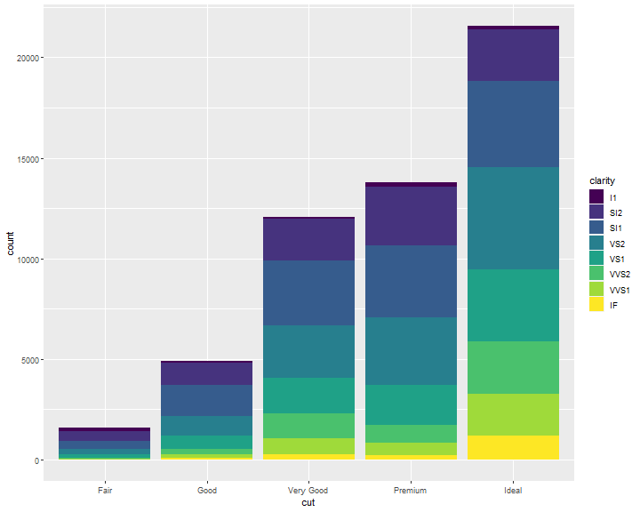
Note what happens if you map the fill aesthetic to another variable, like clarity: the bars are automatically stacked. Each colored rectangle represents a combination of cut and clarity:
ggplot(data = diamonds) +
  geom_bar(mapping = aes(x = cut, fill = clarity))
Position Adjustments: identity
position = "identity" will place each object exactly where it falls in the context of the graph.
This is not very useful for bars, because it overlaps them.
ggplot(data = diamonds,
       mapping = aes(x = cut, fill = clarity)) +
       geom_bar(position = "identity")

To be clearer, we change the transparancy of the bars.
ggplot(data = diamonds,
       mapping = aes(x = cut, fill = clarity)) +
       geom_bar(alpha=1/5,position = "identity")
Did you notice that some of the bars are overlaping?

Therefore, we need to be careful with identity.
You may use the following methods to fix this issue.
Position Adjustments: fill
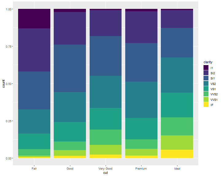
position = "fill" works like stacking, but makes each set of stacked bars the same height. This makes it easier to compare proportions across groups:
ggplot(data = diamonds) +
  geom_bar(mapping = aes(x = cut, fill = clarity),
  position = "fill")
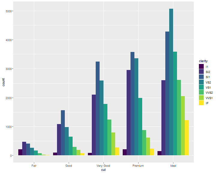
Position Adjustments: dodge
position = "dodge" places overlapping objects directly beside one another. This makes it easier to compare individual values:
ggplot(data = diamonds) +
  geom_bar(mapping = aes(x = cut, fill = clarity),
  position = "dodge")
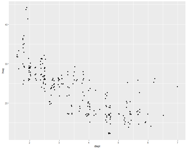
Position Adjustments: jitter
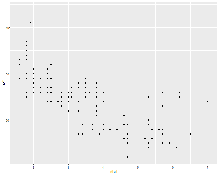
There’s one other type of adjustment that’s not useful for bar charts, but it can be very useful for scatterplots. Recall our first scatterplot. Did you notice that the plot displays only 126 points, even though there are 234 observations in the dataset?
ggplot(data = mpg) +
  geom_point(mapping = aes(x = displ, y = hwy))
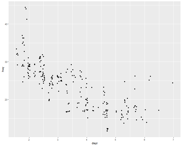
position = "jitter" adds a small amount of random noise to each point. This spreads the points out because no two points are likely to receive the same amount of random noise:
ggplot(data = mpg) +
  geom_point(mapping = aes(x = displ, y = hwy),
  position = "jitter")
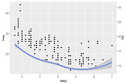
Dual y axis
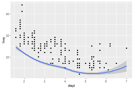
Two y variables with one y axis, the cty is shifted down.
ggplot(data = mpg) +
  geom_point(mapping = aes(x = displ, y = hwy)) +
  geom_smooth(mapping = aes(x = displ, y = cty))
sec_axis() function is able to deal with dual axis
ggplot(data = mpg) +
  geom_point(mapping = aes(x = displ, y = hwy)) +
  geom_smooth(mapping = aes(x = displ, y = cty))+
    scale_y_continuous(sec.axis = sec_axis(~.*0.7, name = "cty"))
Coordinate Systems
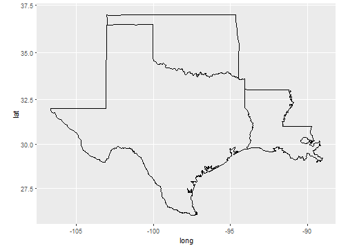
Coordinate systems are probably the most complicated part of ggplot2. The default coordinate system is the Cartesian coordinate system where the x and y position act independently to find the location of each point.
# first: install.packages(c("maps","mapproj")) ----
# then ----
sw <- map_data("state",
               region = c("texas",
                          "oklahoma",
                          "louisiana"))
ggplot(sw) +
  geom_polygon(
    mapping = aes(x = long,
                  y = lat,
                  group = group),
    fill = NA,
    color = "black"
  ) +
  coord_map()
But what if we don't have geocode information
- ggmap package will return geocodes from cities' name. However, as of mid-2018, google map requires a registered API key, which needs a valid credit card (SAD!).
- Therefore, we have to find an altervative way. You could find geocodes data table included cities name on: census.gov or other open liscence sources, e.g. ods.
Then, how to connect geocode table with our original data table by using base function?
Merge geocode with city's name or zip or both
cities <-
  data.frame(
    City = c("Boston", "Newton", "Cambridge"),
    Zip = c(2110, 28658, 5444)
  )
gcode <-
  read.csv("E:/IE6600/materials/R/R/hwData/usZipGeo.csv", sep = ";")
newCities <-
  merge(cities, gcode, by.x = c("City", "Zip")) %>%
  subset(select = c("City", "Zip", "Longitude", "Latitude"))
newCities
##        City   Zip Longitude Latitude
## 1    Boston  2110 -71.05365 42.35653
## 2 Cambridge  5444 -72.90151 44.64565
## 3    Newton 28658 -81.23443 35.65344
Coordinate Systems: polar
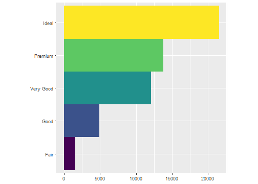
For example, first we do a barchart based on the diamonds dataset.
ggplot(data = diamonds) +
  geom_bar(
    mapping = aes(x = cut, fill = cut),
    show.legend = FALSE,
    width = 1
  ) +
  theme(aspect.ratio = 1) +
  labs(x = NULL, y = NULL)+
  coord_flip()
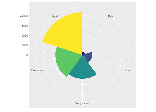
Then we convert it to a polar system by using coord_polar().
ggplot(data = diamonds) +
  geom_bar(
    mapping = aes(x = cut, fill = cut),
    show.legend = FALSE,
    width = 1
  ) +
  theme(aspect.ratio = 1) +
  labs(x = NULL, y = NULL)+
  coord_polar()
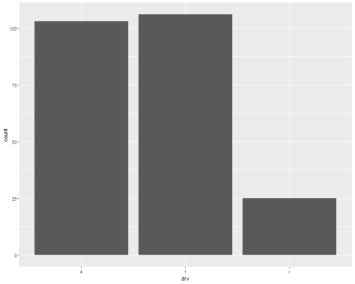
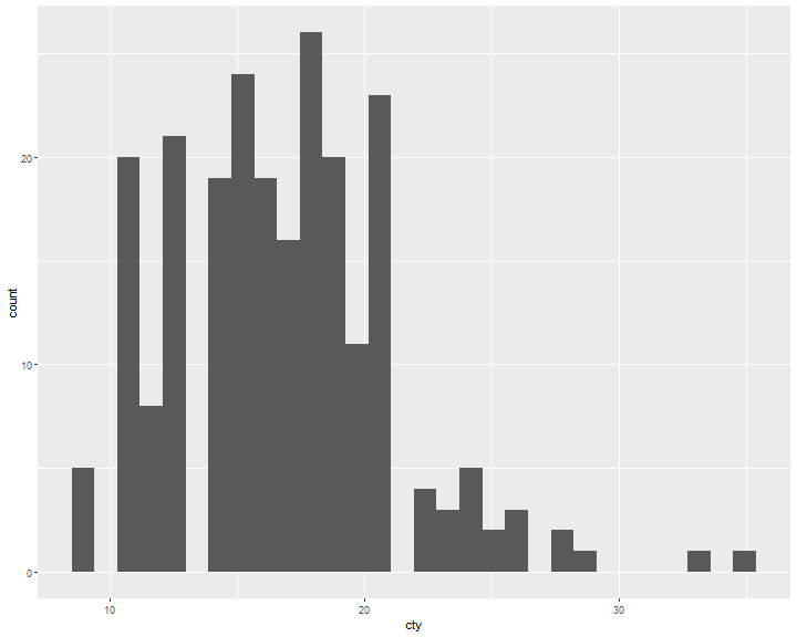
Bar chart vs Histogram
ggplot(data = mpg, mapping = aes(x=drv)) +
    geom_bar()
ggplot(data = mpg, mapping = aes(x=cty)) +
  geom_histogram()
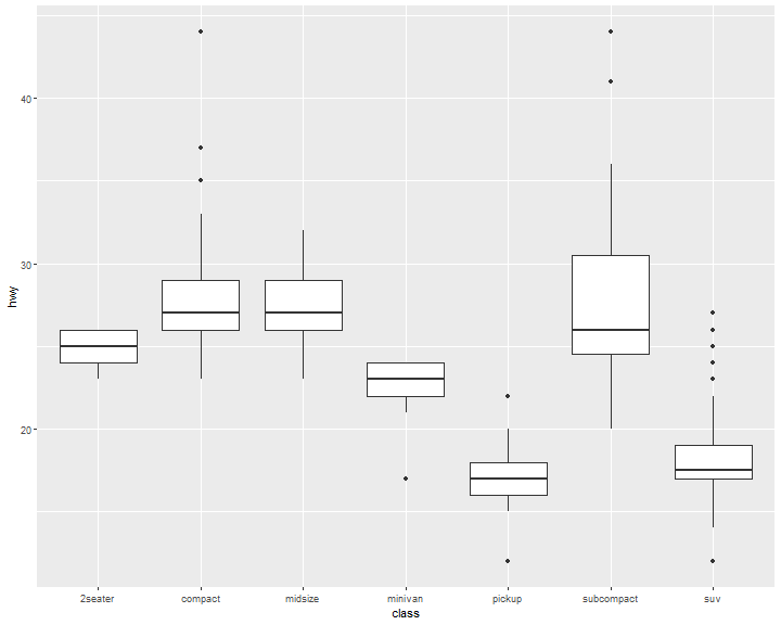
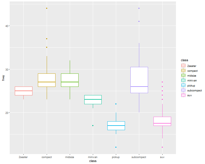
Boxplot
ggplot(data = mpg, mapping = aes(x = class, y = hwy)) +
  geom_boxplot()
ggplot(data = mpg, mapping = aes(x = class, y = hwy)) +
  geom_boxplot(aes(color=class))
Scatter plot
ggplot(data = mpg,
       mapping = aes(x = displ, y = hwy)) +
       geom_point()

Jitter
ggplot(data = mpg,
       mapping = aes(x = displ, y = hwy)) +
       geom_point(position = "jitter")
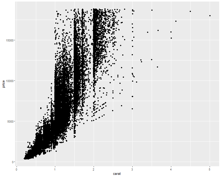
Avoid overlapping
ggplot(diamonds, mapping = aes(x = carat, y = price)) +
  geom_point()
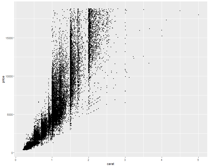
Avoid overlapping: Change size
ggplot(diamonds, mapping=aes(x=carat, y=price)) +
  geom_point(size=0.1)
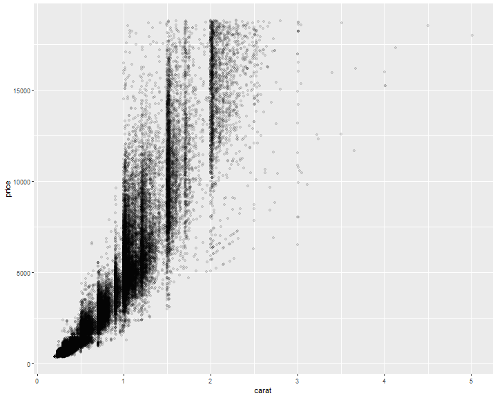
Avoid overlapping: Change alpha
ggplot(diamonds, mapping=aes(x=carat, y=price)) +
  geom_point(alpha=0.1)
References
[1] Dr. Andrew Abela, Choosing a good chart
[2] Hadley Wickham, Garrett Grolemund. R For Data Science.
[3] Hadley Wickham, A layered grammar of graphics
[4] Winston Chang, R Graphics Cookbook
Data Transformation with dplyr
Often you’ll need to create some new variables or summaries, or maybe you just want to rename the variables or reorder the observations in order to make the data a little easier to work with.
# Needed libraries ----
library(nycflights13)
library(dplyr)
#or ----
library(tidyverse)

The conflict message tells you some of the other functions have been overwrited by Tidyverse. If you want to use the base version of these functions after loading dplyr, you’ll need to use their full names: stats::filter() and stats::lag(),etc.
search()
search()
##  [1] ".GlobalEnv"           "package:forcats"      "package:stringr"
##  [4] "package:dplyr"        "package:purrr"        "package:readr"
##  [7] "package:tidyr"        "package:tibble"       "package:ggplot2"
## [10] "package:tidyverse"    "package:nycflights13" "package:stats"
## [13] "package:graphics"     "package:grDevices"    "package:utils"
## [16] "package:datasets"     "package:methods"      "Autoloads"
## [19] "package:base"
You may use the full syntax package::function_name() to load the specific function, if there are any overwriting issues occured.
Package nycflights13
To explore the basic data manipulation verbs of dplyr, we’ll use nycflights13::flights. This data frame contains all 336,776 flights that departed from New York City in 2013:
head(flights)
## # A tibble: 6 × 19
##    year month   day dep_time sched_dep_time dep_delay arr_time sched_arr_time
##   <int> <int> <int>    <int>          <int>     <dbl>    <int>          <int>
## 1  2013     1     1      517            515         2      830            819
## 2  2013     1     1      533            529         4      850            830
## 3  2013     1     1      542            540         2      923            850
## 4  2013     1     1      544            545        -1     1004           1022
## 5  2013     1     1      554            600        -6      812            837
## 6  2013     1     1      554            558        -4      740            728
## # … with 11 more variables: arr_delay <dbl>, carrier <chr>, flight <int>,
## #   tailnum <chr>, origin <chr>, dest <chr>, air_time <dbl>, distance <dbl>,
## #   hour <dbl>, minute <dbl>, time_hour <dttm>
Interview data with view()
view(flights)
You might also have noticed the row of three- (or four-) letter abbreviations under the column names. These describe the type of each variable:
- int stands for integers.
- dbl stands for doubles, or real numbers.
- chr stands for character vectors, or strings.
- dttm stands for date-times (a date + a time).
Flights actually is a tibble, a special type of data.frame. We will talk about it later.
There are three other common types of variables that aren’t used in this dataset but you’ll encounter later.
- lgl stands for logical, vectors that contain only TRUE or FALSE.
- fctr stands for factors, which R uses to represent categorical variables with fixed possible values.
- date stands for dates.
dplyr
You are going to learn the five key dplyr functions that allow you to solve the vast majority of your data-manipulation challenges:
filter()pick observations by their values .arrange()Reorder the rows.select()Pick variables by their names.mutate()Create new variables with functions of existing variables.summarize()Collapse many values down to a single summary.group_by()Conjunction.
dplyr grammar
All verbs work similarly: filter(df, argument,...)
- The first argument is a data frame.
- The subsequent arguments describe what to do with the data frame, using the variable names (without quotes).
- The result is a new data frame.
filter()
Filter rows with filter()
filter() allows you to subset observations based on their values.
Base function in R:
flights[flights$month==1&flights$day==1,]
filter() function in dplyr:
filter(flights, month==1,day==1)
We only want to see the Jan.1st flights
jan <- filter(flights, month==1, day==1)
jan
## # A tibble: 842 × 19
##     year month   day dep_time sched_dep_time dep_delay arr_time sched_arr_time
##    <int> <int> <int>    <int>          <int>     <dbl>    <int>          <int>
##  1  2013     1     1      517            515         2      830            819
##  2  2013     1     1      533            529         4      850            830
##  3  2013     1     1      542            540         2      923            850
##  4  2013     1     1      544            545        -1     1004           1022
##  5  2013     1     1      554            600        -6      812            837
##  6  2013     1     1      554            558        -4      740            728
##  7  2013     1     1      555            600        -5      913            854
##  8  2013     1     1      557            600        -3      709            723
##  9  2013     1     1      557            600        -3      838            846
## 10  2013     1     1      558            600        -2      753            745
## # … with 832 more rows, and 11 more variables: arr_delay <dbl>, carrier <chr>,
## #   flight <int>, tailnum <chr>, origin <chr>, dest <chr>, air_time <dbl>,
## #   distance <dbl>, hour <dbl>, minute <dbl>, time_hour <dttm>
Filter rows with filter(): examples
dec25 <- filter(flights, month == 12, day == 25)
dec25
## # A tibble: 719 × 19
##     year month   day dep_time sched_dep_time dep_delay arr_time sched_arr_time
##    <int> <int> <int>    <int>          <int>     <dbl>    <int>          <int>
##  1  2013    12    25      456            500        -4      649            651
##  2  2013    12    25      524            515         9      805            814
##  3  2013    12    25      542            540         2      832            850
##  4  2013    12    25      546            550        -4     1022           1027
##  5  2013    12    25      556            600        -4      730            745
##  6  2013    12    25      557            600        -3      743            752
##  7  2013    12    25      557            600        -3      818            831
##  8  2013    12    25      559            600        -1      855            856
##  9  2013    12    25      559            600        -1      849            855
## 10  2013    12    25      600            600         0      850            846
## # … with 709 more rows, and 11 more variables: arr_delay <dbl>, carrier <chr>,
## #   flight <int>, tailnum <chr>, origin <chr>, dest <chr>, air_time <dbl>,
## #   distance <dbl>, hour <dbl>, minute <dbl>, time_hour <dttm>
filter() - comparison
To use filtering effectively, you have to know how to select the observations that you want using the comparison operators.
R provides the standard suite: >, >=, <, <=, != (not equal), and == (equal).
Flights on Feb~Dec, and before 28 th
filter(flights, month>1&!day>28)
Flights on Feb~Dec, and before 28 th
flights28 <- filter(flights, month>1&!day>28)
flights28
## # A tibble: 285,972 × 19
##     year month   day dep_time sched_dep_time dep_delay arr_time sched_arr_time
##    <int> <int> <int>    <int>          <int>     <dbl>    <int>          <int>
##  1  2013    10     1      447            500       -13      614            648
##  2  2013    10     1      522            517         5      735            757
##  3  2013    10     1      536            545        -9      809            855
##  4  2013    10     1      539            545        -6      801            827
##  5  2013    10     1      539            545        -6      917            933
##  6  2013    10     1      544            550        -6      912            932
##  7  2013    10     1      549            600       -11      653            716
##  8  2013    10     1      550            600       -10      648            700
##  9  2013    10     1      550            600       -10      649            659
## 10  2013    10     1      551            600        -9      727            730
## # … with 285,962 more rows, and 11 more variables: arr_delay <dbl>,
## #   carrier <chr>, flight <int>, tailnum <chr>, origin <chr>, dest <chr>,
## #   air_time <dbl>, distance <dbl>, hour <dbl>, minute <dbl>, time_hour <dttm>
Tips
When you’re starting out with R, the easiest mistake to make is to use
=instead of==when testing for equality. When this happens you’ll get an informative error:filter(flights, month = 1)## Error in `filter()`: ## ! We detected a named input. ## ℹ This usually means that you've used `=` instead of `==`. ## ℹ Did you mean `month == 1`?There’s another common problem you might encounter when using
==: floating-point numbers.sqrt(2)^2==2## [1] FALSE1/49*49==1## [1] FALSEComputers use finite precision arithmetic (they obviously can’t store an infinite number of digits!) so remember that every number you see is an approximation. Instead of relying on
==, use near():near(sqrt(2) ^ 2, 2)## [1] TRUEnear(1 / 49 * 49, 1)## [1] TRUE
Logical operators
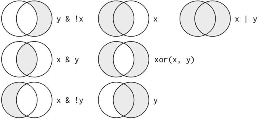
nycflights13: Flights on May or June
mayJune <- filter(flights, month==5|month==6)
mayJune$month %>% unique()
## [1] 5 6
Tips: %in%
A useful shorthand for this problem is x %in% y. This will select every row where x is one of the values in y. We could use it to rewrite the preceding code: Retrieve the flights information on Jan, Feb, and Mar
filter(flights, month%in%c(1,2,3)) %>% head()
!= not equals to
Flights not on Feb
filter(flights, month!=2)
## # A tibble: 311,825 × 19
##     year month   day dep_time sched_dep_time dep_delay arr_time sched_arr_time
##    <int> <int> <int>    <int>          <int>     <dbl>    <int>          <int>
##  1  2013     1     1      517            515         2      830            819
##  2  2013     1     1      533            529         4      850            830
##  3  2013     1     1      542            540         2      923            850
##  4  2013     1     1      544            545        -1     1004           1022
##  5  2013     1     1      554            600        -6      812            837
##  6  2013     1     1      554            558        -4      740            728
##  7  2013     1     1      555            600        -5      913            854
##  8  2013     1     1      557            600        -3      709            723
##  9  2013     1     1      557            600        -3      838            846
## 10  2013     1     1      558            600        -2      753            745
## # … with 311,815 more rows, and 11 more variables: arr_delay <dbl>,
## #   carrier <chr>, flight <int>, tailnum <chr>, origin <chr>, dest <chr>,
## #   air_time <dbl>, distance <dbl>, hour <dbl>, minute <dbl>, time_hour <dttm>
|, &, and ","
Compare the following three code chunks
filter(flights, !(arr_delay > 120 | dep_delay > 120)) %>%
  select(dep_delay) %>% head(3)
filter(flights, arr_delay <= 120, dep_delay <= 120) %>%
  select(dep_delay) %>% head(3)
filter(flights, !arr_delay > 120 & !dep_delay > 120) %>%
  select(dep_delay) %>% head(3)
## # A tibble: 3 × 1
##   dep_delay
##       <dbl>
## 1         2
## 2         4
## 3         2
Missing Values
One important feature of R that can make comparison tricky is missing values, or NAs (“not availables”).
NA>5
## [1] NA
NA==10
## [1] NA
NA+10
## [1] NA
NA/2
[1] NA
### NA==NA

The most confusing result is this one:

```r
NA==NA
## [1] NA
But we can understand it easily in one example:
# Let ZAge be Zhenyuan's age. We don't know how old he is.
ZAge <- NA
# Let TAge be one random Tub's age. We don't know how old they is. (Pretty sure we don't know a random Tub's age...)
TAge <- NA
# Are Zhenyuan and Tub the same age?
ZAge == TAge
## [1] NA
# We don't know!
NA with filter()
filter() only includes rows where the condition is TRUE;
it excludes both FALSE and NA values.
If you want to preserve missing values, ask for them explicitly:
df <- tibble(x = c(1, NA, 3))
filter(df, x > 1)
## # A tibble: 1 × 1
##       x
##   <dbl>
## 1     3
filter(df, is.na(x) | x > 1)
## # A tibble: 2 × 1
##       x
##   <dbl>
## 1    NA
## 2     3
Some other functions
is.na(NA)
## [1] TRUE
df <- data.frame(A=c(1,NA,2))

na.omit(df)
##   A
## 1 1
## 3 2
sum(df[,1], na.rm=T)
## [1] 3
Exercise 1
Find all flights that:
Flew to Houston (IAH)
Were operated by United (UA), American (AA), or Delta (DL)
Departed in summer (July, August, and September)
Exercise 2
Use data set msleep, and create a new data frame of mammals with feeding type carnivore and brain weight less than the average of brain weight over all mammals. Make sure no NA values in column of brain weight.
arrange()
Arrange Rows with arrange()
arrange() works similarly to filter() except that instead of selecting rows, it changes their order
Base function in R:
flights[order(flights$year,flights$month, flights$day, decreasing=F),]
arrange() function in dplyr:
arrange(flights, year, month, day)
## # A tibble: 336,776 × 19
##     year month   day dep_time sched_dep_time dep_delay arr_time sched_arr_time
##    <int> <int> <int>    <int>          <int>     <dbl>    <int>          <int>
##  1  2013     1     1      517            515         2      830            819
##  2  2013     1     1      533            529         4      850            830
##  3  2013     1     1      542            540         2      923            850
##  4  2013     1     1      544            545        -1     1004           1022
##  5  2013     1     1      554            600        -6      812            837
##  6  2013     1     1      554            558        -4      740            728
##  7  2013     1     1      555            600        -5      913            854
##  8  2013     1     1      557            600        -3      709            723
##  9  2013     1     1      557            600        -3      838            846
## 10  2013     1     1      558            600        -2      753            745
## # … with 336,766 more rows, and 11 more variables: arr_delay <dbl>,
## #   carrier <chr>, flight <int>, tailnum <chr>, origin <chr>, dest <chr>,
## #   air_time <dbl>, distance <dbl>, hour <dbl>, minute <dbl>, time_hour <dttm>
Use desc() to reorder by a column in descending order
arrange(flights, desc(arr_delay))
## # A tibble: 336,776 × 19
##     year month   day dep_time sched_dep_time dep_delay arr_time sched_arr_time
##    <int> <int> <int>    <int>          <int>     <dbl>    <int>          <int>
##  1  2013     1     9      641            900      1301     1242           1530
##  2  2013     6    15     1432           1935      1137     1607           2120
##  3  2013     1    10     1121           1635      1126     1239           1810
##  4  2013     9    20     1139           1845      1014     1457           2210
##  5  2013     7    22      845           1600      1005     1044           1815
##  6  2013     4    10     1100           1900       960     1342           2211
##  7  2013     3    17     2321            810       911      135           1020
##  8  2013     7    22     2257            759       898      121           1026
##  9  2013    12     5      756           1700       896     1058           2020
## 10  2013     5     3     1133           2055       878     1250           2215
## # … with 336,766 more rows, and 11 more variables: arr_delay <dbl>,
## #   carrier <chr>, flight <int>, tailnum <chr>, origin <chr>, dest <chr>,
## #   air_time <dbl>, distance <dbl>, hour <dbl>, minute <dbl>, time_hour <dttm>
Missing values are always sorted at the end
df <- data.frame(x = c(5, 2, NA))
arrange(df, x) #or arrange(df, desc(x))
##    x
## 1  2
## 2  5
## 3 NA
Exercises
- Sort flights to find the most delayed flights. Find the flights that left earliest.
- Sort flights to find the fastest flights.
select()
Select Columns with select()
select() allows you to rapidly zoom in on a useful subset using operations based on the names of the variables.
Base function in R:
# Select columns by name
flights[,c("year","month","day")]
select() function in dplyr:
# Select columns by name
select(flights, year, month, day)
## # A tibble: 336,776 × 3
##     year month   day
##    <int> <int> <int>
##  1  2013     1     1
##  2  2013     1     1
##  3  2013     1     1
##  4  2013     1     1
##  5  2013     1     1
##  6  2013     1     1
##  7  2013     1     1
##  8  2013     1     1
##  9  2013     1     1
## 10  2013     1     1
## # … with 336,766 more rows
Select all colums between year and day
select(flights, year:day)
## # A tibble: 336,776 × 3
##     year month   day
##    <int> <int> <int>
##  1  2013     1     1
##  2  2013     1     1
##  3  2013     1     1
##  4  2013     1     1
##  5  2013     1     1
##  6  2013     1     1
##  7  2013     1     1
##  8  2013     1     1
##  9  2013     1     1
## 10  2013     1     1
## # … with 336,766 more rows
Select all columns except those from year to day
select(flights, -(year:day))
## # A tibble: 336,776 × 16
##    dep_time sched_dep_time dep_delay arr_time sched_arr_time arr_delay carrier
##       <int>          <int>     <dbl>    <int>          <int>     <dbl> <chr>
##  1      517            515         2      830            819        11 UA
##  2      533            529         4      850            830        20 UA
##  3      542            540         2      923            850        33 AA
##  4      544            545        -1     1004           1022       -18 B6
##  5      554            600        -6      812            837       -25 DL
##  6      554            558        -4      740            728        12 UA
##  7      555            600        -5      913            854        19 B6
##  8      557            600        -3      709            723       -14 EV
##  9      557            600        -3      838            846        -8 B6
## 10      558            600        -2      753            745         8 AA
## # … with 336,766 more rows, and 9 more variables: flight <int>, tailnum <chr>,
## #   origin <chr>, dest <chr>, air_time <dbl>, distance <dbl>, hour <dbl>,
## #   minute <dbl>, time_hour <dttm>
Other arguments within select()
There are a number of helper functions you can use within select():
starts_with("abc")matches names that begin with “abc”.ends_with("xyz")matches names that end with “xyz”.contains("ijk")matches names that contain “ijk”.matches("^a")selects variables that match a regular expression. (check R4DS "regular expressions")num_range("x", 1:3)matches x1, x2, and x3.
select(): examples
abc.df <- data.frame(apple=c("b", "c"), an.orange=1:2, orange1=2:3)
abc.df
##   apple an.orange orange1
## 1     b         1       2
## 2     c         2       3
select(abc.df, starts_with("app"))
##   apple
## 1     b
## 2     c
select(abc.df, ends_with("ge"))
##   an.orange
## 1         1
## 2         2
select(abc.df, contains("pp"))
##   apple
## 1     b
## 2     c
select(abc.df, matches("^a"))
##   apple an.orange
## 1     b         1
## 2     c         2
select(abc.df, num_range("orange", 1))
##   orange1
## 1       2
## 2       3
mutate()
Add New Variables with mutate()
References
[1] Hadley Wickham, Garrett Grolemund. R For Data Science.
Data wrangling with tibbles, readr and tidyr
Where are we (probability 0.8)
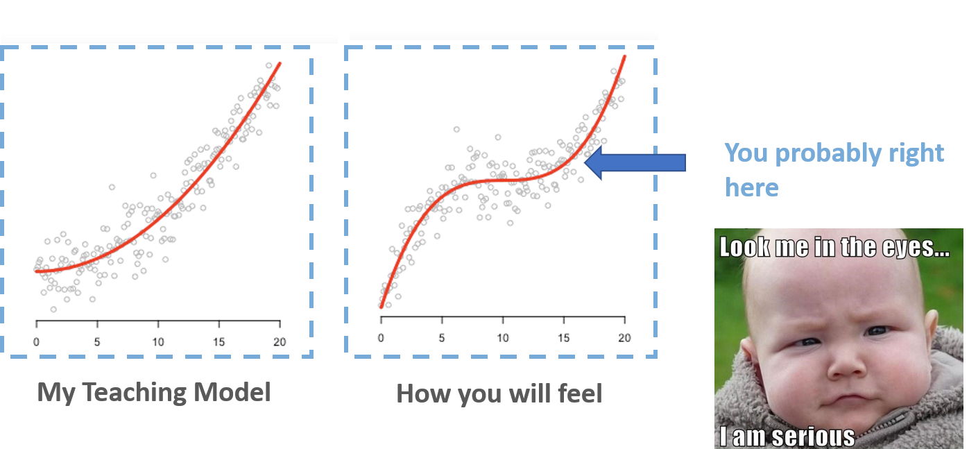
Tibbles with tibble
Tibble and Prerequisites
Tibbles are a modern take on data frames. They keep the features that have stood the test of time, and drop the features that used to be convenient but are now frustrating (i.e. converting character vectors to factors).
library(tidyverse)
#or
library(tibble)
Packages/Books Authors
Dr. Hadley Wickham
- Chief Scientist at RStudio,
- Adjunct Professor of Statistics at University of Auckland, Stanford University, and Rice University
- Books: R for Data Science, Advanced R, R packages
- Packages: tidyverse, devtools, pkgdown
Dr. Yihui Xie
- SDE at RStudio
- Packages: knitr, rmarkdown, shiny, tinytex, bookdown, DT
Tips
If you wanted to learn more about the packages from tidyverse, you may try
  vignette("tibble")
  vignette("ggplot2-specs")
Pronounce [vin'jet]
Creating tibbles
tibble() is a nice way to create data frames. It encapsulates best practices for data frames:
tibble(letter=c("a","b","c"), number=c(1:3))
## # A tibble: 3 × 2
##   letter number
##   <chr>   <int>
## 1 a           1
## 2 b           2
## 3 c           3
Convert the data frame into tibble version of data frame
You can do that with as_tibble():
irisTibble <- as_tibble(iris)
class(irisTibble)
Adjust the names of variables
data.frame() will adjust the name of variables, unless overwrite check.names=F
data.frame(`a b`=c(1:3))
##   a.b
## 1   1
## 2   2
## 3   3
data.frame(`a b`=c(1:3), check.names = F)
##   a b
## 1   1
## 2   2
## 3   3
tibble() never adjusts the name of variables
tibble(`a b`=c(1:3))
## # A tibble: 3 × 1
##   `a b`
##   <int>
## 1     1
## 2     2
## 3     3
tibble() never adjusts the name of variables: Nonsyntactic names
It’s possible for a tibble to have column names that are not valid R variable names, aka nonsyntactic names.
data.frame(
  `:(` = "unhappy",
  ` ` = "space",
  `2000` = "number"
)
##       X..    X.  X2000
## 1 unhappy space number
tibble(
  `:(` = "unhappy",
  ` ` = "space",
  `2000` = "number"
)
## # A tibble: 1 × 3
##   `:(`    ` `   `2000`
##   <chr>   <chr> <chr>
## 1 unhappy space number
Arguments
tibble(x=1:3,
       y=x^2)
## # A tibble: 3 × 2
##       x     y
##   <int> <dbl>
## 1     1     1
## 2     2     4
## 3     3     9
Creating with tribble()
Another way to create a tibble is with tribble(), short for transposed tibble. tribble() is customized for data entry in code: column headings are defined by formulas (i.e., they start with ~), and entries are separated by commas. This makes it possible to lay out small amounts of data in easy-to-read form:
tribble(~x, ~y, ~z,
        "a", 1, 3.5,
        "b", 2, 3)
## # A tibble: 2 × 3
##   x         y     z
##   <chr> <dbl> <dbl>
## 1 a         1   3.5
## 2 b         2   3
Data import with readr
readr and prerequisites
Here we will only introduce the most common function from the readr package read_csv()
library(tidyverse)
#or
library(readr)
Compared to the Base R function read.csv()
- They are typically much faster (~10x)
- They produce tibbles, and they don’t convert character vectors to factors, use row names, or munge the column names.
- They are more reproducible.
Reading csv with read_csv()
df1 <-
  read_csv(
    "https://gist.githubusercontent.com/omarish/5687264/raw/7e5c814ce6ef33e25d5259c1fe79463c190800d9/mpg.csv"
  )
df2 <- read_csv(readr_example("mtcars.csv"))
df1 <-
read_csv(
"https://gist.githubusercontent.com/omarish/5687264/raw/7e5c814ce6ef33e25d5259c1fe79463c190800d9/mpg.csv"
)
## Rows: 398 Columns: 9
## ── Column specification ────────────────────────────────────────────────────────
## Delimiter: ","
## chr (2): horsepower, name
## dbl (7): mpg, cylinders, displacement, weight, acceleration, model_year, origin
##
## ℹ Use `spec()` to retrieve the full column specification for this data.
## ℹ Specify the column types or set `show_col_types = FALSE` to quiet this message.
df1
## # A tibble: 398 × 9
## mpg cylinders displacement horsepower weight acceleration model_year origin
## <dbl> <dbl> <dbl> <chr> <dbl> <dbl> <dbl> <dbl>
## 1 18 8 307 130 3504 12 70 1
## 2 15 8 350 165 3693 11.5 70 1
## 3 18 8 318 150 3436 11 70 1
## 4 16 8 304 150 3433 12 70 1
## 5 17 8 302 140 3449 10.5 70 1
## 6 15 8 429 198 4341 10 70 1
## 7 14 8 454 220 4354 9 70 1
## 8 14 8 440 215 4312 8.5 70 1
## 9 14 8 455 225 4425 10 70 1
## 10 15 8 390 190 3850 8.5 70 1
## # … with 388 more rows, and 1 more variable: name <chr>
df2 <- read_csv(readr_example("mtcars.csv"))
## Rows: 32 Columns: 11
## ── Column specification ────────────────────────────────────────────────────────
## Delimiter: ","
## dbl (11): mpg, cyl, disp, hp, drat, wt, qsec, vs, am, gear, carb
##
## ℹ Use `spec()` to retrieve the full column specification for this data.
## ℹ Specify the column types or set `show_col_types = FALSE` to quiet this message.
df2
## # A tibble: 32 × 11
## mpg cyl disp hp drat wt qsec vs am gear carb
## <dbl> <dbl> <dbl> <dbl> <dbl> <dbl> <dbl> <dbl> <dbl> <dbl> <dbl>
## 1 21 6 160 110 3.9 2.62 16.5 0 1 4 4
## 2 21 6 160 110 3.9 2.88 17.0 0 1 4 4
## 3 22.8 4 108 93 3.85 2.32 18.6 1 1 4 1
## 4 21.4 6 258 110 3.08 3.22 19.4 1 0 3 1
## 5 18.7 8 360 175 3.15 3.44 17.0 0 0 3 2
## 6 18.1 6 225 105 2.76 3.46 20.2 1 0 3 1
## 7 14.3 8 360 245 3.21 3.57 15.8 0 0 3 4
## 8 24.4 4 147. 62 3.69 3.19 20 1 0 4 2
## 9 22.8 4 141. 95 3.92 3.15 22.9 1 0 4 2
## 10 19.2 6 168. 123 3.92 3.44 18.3 1 0 4 4
## # … with 22 more rows
Like tribble(), inline input is also accepted.
read_csv("x, y, z
1, 1, 1
2, 2, 2")
## Rows: 2 Columns: 3
## ── Column specification ────────────────────────────────────────────────────────
## Delimiter: ","
## dbl (3): x, y, z
##
## ℹ Use `spec()` to retrieve the full column specification for this data.
## ℹ Specify the column types or set `show_col_types = FALSE` to quiet this message.
## # A tibble: 2 × 3
## x y z
## <dbl> <dbl> <dbl>
## 1 1 1 1
## 2 2 2 2
Replace values with NA
read_csv("x, y, z
1, 1, 1
2, 2, 2", na="1")
## Rows: 2 Columns: 3
## ── Column specification ────────────────────────────────────────────────────────
## Delimiter: ","
## dbl (3): x, y, z
##
## ℹ Use `spec()` to retrieve the full column specification for this data.
## ℹ Specify the column types or set `show_col_types = FALSE` to quiet this message.
## # A tibble: 2 × 3
## x y z
## <dbl> <dbl> <dbl>
## 1 NA NA NA
## 2 2 2 2
Let's recall the example of h1b data in hw2
When we use the base function read.csv, the parse of data types may be wrong:
h1b19 <-
read.csv("E:/IE6600/materials/assignment/hw/hw2/h1b_datahubexport-2019.csv")
sapply(h1b19[, 3:6], class)
## Initial.Approvals Initial.Denials Continuing.Approvals
## "character" "character" "character"
## Continuing.Denials
## "character"
guess_max
The default guesses are only for the first 1000 rows. Sometimes, 1000 rows may not be enough for read_csv() to parse the column specification. We could use guess_max= to increase the guessing rows.
chg <- read_csv(readr_example("challenge.csv"))
## Rows: 2000 Columns: 2
## ── Column specification ────────────────────────────────────────────────────────
## Delimiter: ","
## dbl (1): x
## date (1): y
##
## ℹ Use `spec()` to retrieve the full column specification for this data.
## ℹ Specify the column types or set `show_col_types = FALSE` to quiet this message.
adj.chg<- read_csv(readr_example("challenge.csv"), guess_max = 1500)
Compared to default read.csv
adj.chg2<- read.csv(readr_example("challenge.csv"))
class(adj.chg2$y[1])
## [1] "character"
class(adj.chg$y[1])
## [1] "Date"
Two cases 1/2
Sometimes there are a few lines of metadata at the top of the file. You can use skip = n to skip the first n lines; or use comment = "#" to drop all lines that start with (e.g.) #:
read_csv("# A comment I want to skip
x,y,z
1,2,3", comment = "#")
## Rows: 1 Columns: 3
## ── Column specification ────────────────────────────────────────────────────────
## Delimiter: ","
## dbl (3): x, y, z
##
## ℹ Use `spec()` to retrieve the full column specification for this data.
## ℹ Specify the column types or set `show_col_types = FALSE` to quiet this message.
## # A tibble: 1 × 3
## x y z
## <dbl> <dbl> <dbl>
## 1 1 2 3
Two cases 2/2
The data might not have column names. You can use col_names = FALSE to tell read_csv() not to treat the first row as headings, and instead label them sequentially from X1 to Xn:
read_csv("1,2,3\n4,5,6", col_names = FALSE)
## Rows: 2 Columns: 3
## ── Column specification ────────────────────────────────────────────────────────
## Delimiter: ","
## dbl (3): X1, X2, X3
##
## ℹ Use `spec()` to retrieve the full column specification for this data.
## ℹ Specify the column types or set `show_col_types = FALSE` to quiet this message.
## # A tibble: 2 × 3
## X1 X2 X3
## <dbl> <dbl> <dbl>
## 1 1 2 3
## 2 4 5 6
read_csv("1,2,3\n4,5,6",col_names = c("x", "y", "z"))
Writing csv with write_csv()
The default syntax:
write_csv(yourDataName, "yourLocation/yourCSVname.csv")
Tidy data with tidyr
Prerequisites
In this chapter we’ll focus on tidyr, a package that provides a bunch of tools to help tidy up your messy datasets. tidyr is a member of the core tidyverse.
library(tidyr)
#or
library(tidyverse)
Five data tables we will use from the packages tidyverse:
table1, table2, table3, table4a, table4b
What is tidy data?
There are three interrelated rules which make a dataset tidy:
- Each variable must have its own column.
- Each observation must have its own row.
- Each value must have its own cell.

What do you think of this data? Tidy?
## # A tibble: 12 × 4
## country year type count
## <chr> <int> <chr> <int>
## 1 Afghanistan 1999 cases 745
## 2 Afghanistan 1999 population 19987071
## 3 Afghanistan 2000 cases 2666
## 4 Afghanistan 2000 population 20595360
## 5 Brazil 1999 cases 37737
## 6 Brazil 1999 population 172006362
## 7 Brazil 2000 cases 80488
## 8 Brazil 2000 population 174504898
## 9 China 1999 cases 212258
## 10 China 1999 population 1272915272
## 11 China 2000 cases 213766
## 12 China 2000 population 1280428583
## # A tibble: 6 × 3
## country year rate
## * <chr> <int> <chr>
## 1 Afghanistan 1999 745/19987071
## 2 Afghanistan 2000 2666/20595360
## 3 Brazil 1999 37737/172006362
## 4 Brazil 2000 80488/174504898
## 5 China 1999 212258/1272915272
## 6 China 2000 213766/1280428583
## # A tibble: 3 × 3
## country `1999` `2000`
## * <chr> <int> <int>
## 1 Afghanistan 745 2666
## 2 Brazil 37737 80488
## 3 China 212258 213766
## # A tibble: 3 × 3
## country `1999` `2000`
## * <chr> <int> <int>
## 1 Afghanistan 19987071 20595360
## 2 Brazil 172006362 174504898
## 3 China 1272915272 1280428583
## # A tibble: 6 × 4
## country year cases population
## <chr> <int> <int> <int>
## 1 Afghanistan 1999 745 19987071
## 2 Afghanistan 2000 2666 20595360
## 3 Brazil 1999 37737 172006362
## 4 Brazil 2000 80488 174504898
## 5 China 1999 212258 1272915272
## 6 China 2000 213766 1280428583
## # A tibble: 6 × 4
## country century year rate
## * <chr> <chr> <chr> <chr>
## 1 Afghanistan 19 99 745/19987071
## 2 Afghanistan 20 00 2666/20595360
## 3 Brazil 19 99 37737/172006362
## 4 Brazil 20 00 80488/174504898
## 5 China 19 99 212258/1272915272
## 6 China 20 00 213766/1280428583
Why ensure that your data is tidy?
- Picking one consistent way of storing data.
- Placing variables in columns is intuitively and computationally efficient
Spreading and Gathering
The tidyr packages is one part of the tidyverse To resolve one of the two common problems when dealing with datasets:
- One variable might be spread across multiple columns.
- One observation might be scattered across multiple rows.
We need to use gather() and spread() from tidyr
Gathering
A common problem is a dataset where some of the column names are not names of variables, but values of a variable
table4a
## # A tibble: 3 × 3
## country `1999` `2000`
## * <chr> <int> <int>
## 1 Afghanistan 745 2666
## 2 Brazil 37737 80488
## 3 China 212258 213766
table4a %>%
gather("1999", "2000", key="year", value="cases")
## # A tibble: 6 × 3
## country year cases
## <chr> <chr> <int>
## 1 Afghanistan 1999 745
## 2 Brazil 1999 37737
## 3 China 1999 212258
## 4 Afghanistan 2000 2666
## 5 Brazil 2000 80488
## 6 China 2000 213766
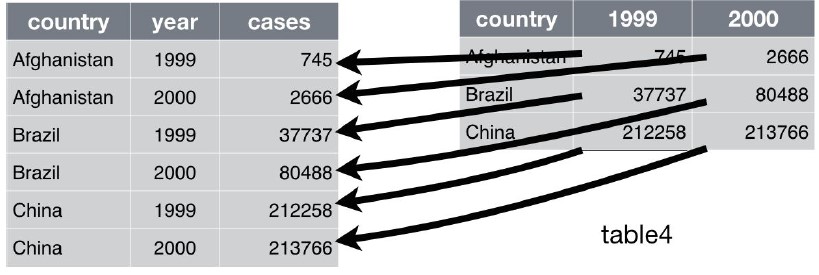
Exercise
use
gather()to make table4b tidytable4b## # A tibble: 3 × 3 ## country `1999` `2000` ## * <chr> <int> <int> ## 1 Afghanistan 19987071 20595360 ## 2 Brazil 172006362 174504898 ## 3 China 1272915272 1280428583Solution:
table4b %>% gather("1999", "2000", key="year", value="population")
Spreading
Spreading is the opposite of gathering. You use it when an observation is scattered across multiple rows.
table2
## # A tibble: 12 × 4
## country year type count
## <chr> <int> <chr> <int>
## 1 Afghanistan 1999 cases 745
## 2 Afghanistan 1999 population 19987071
## 3 Afghanistan 2000 cases 2666
## 4 Afghanistan 2000 population 20595360
## 5 Brazil 1999 cases 37737
## 6 Brazil 1999 population 172006362
## 7 Brazil 2000 cases 80488
## 8 Brazil 2000 population 174504898
## 9 China 1999 cases 212258
## 10 China 1999 population 1272915272
## 11 China 2000 cases 213766
## 12 China 2000 population 1280428583
table2 %>%
spread(key=type, value=count)
## # A tibble: 6 × 4
## country year cases population
## <chr> <int> <int> <int>
## 1 Afghanistan 1999 745 19987071
## 2 Afghanistan 2000 2666 20595360
## 3 Brazil 1999 37737 172006362
## 4 Brazil 2000 80488 174504898
## 5 China 1999 212258 1272915272
## 6 China 2000 213766 1280428583
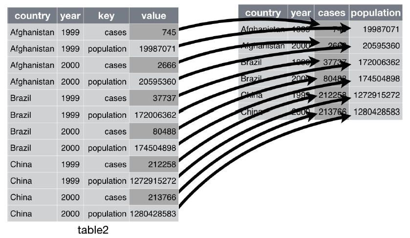
Exercise I
Use
tribble()ortibble()create a data table as follows:## # A tibble: 2 × 3 ## pregnant male female ## <chr> <dbl> <dbl> ## 1 yes NA 10 ## 2 no 20 12Then make it tidy.
Solution:
tribble(~pregnant, ~male, ~female, "yes", NA, 10, "no", 20, 12 ) %>% gather(male, female, key="gender", value="pop")
Exercise II
Use tribble() or tibble() create a data table as follows:
## # A tibble: 6 × 3 ## person index number ## <chr> <chr> <dbl> ## 1 A weight(kg) 52.5 ## 3 C weight(kg) 54.6 ## 4 A height(cm) 179. ## 5 B height(cm) 171. ## 6 C height(cm) 173.Then make it tidy.
Solution:
tibble(person=rep(c("A","B","C"),2), index=c(rep("weight(kg)",3),rep("height(cm)",3)), number=rd) %>% spread(key=index, value=number)
Separating and Pull
So far you’ve learned how to tidy table2 and table4, but not table3. table3 has a different problem: we have one column (rate) that contains two variables (cases and population). To fix this problem, we’ll need the separate() function.
Separate
separate() pulls apart one column into multiple columns, by splitting wherever a separator character appears.
table3
## # A tibble: 6 × 3
## country year rate
## * <chr> <int> <chr>
## 1 Afghanistan 1999 745/19987071
## 2 Afghanistan 2000 2666/20595360
## 3 Brazil 1999 37737/172006362
## 4 Brazil 2000 80488/174504898
## 5 China 1999 212258/1272915272
## 6 China 2000 213766/1280428583
table3 %>%
separate(rate, into=c("cases","population"))
## # A tibble: 6 × 4
## country year cases population
## <chr> <int> <chr> <chr>
## 1 Afghanistan 1999 745 19987071
## 2 Afghanistan 2000 2666 20595360
## 3 Brazil 1999 37737 172006362
## 4 Brazil 2000 80488 174504898
## 5 China 1999 212258 1272915272
## 6 China 2000 213766 1280428583
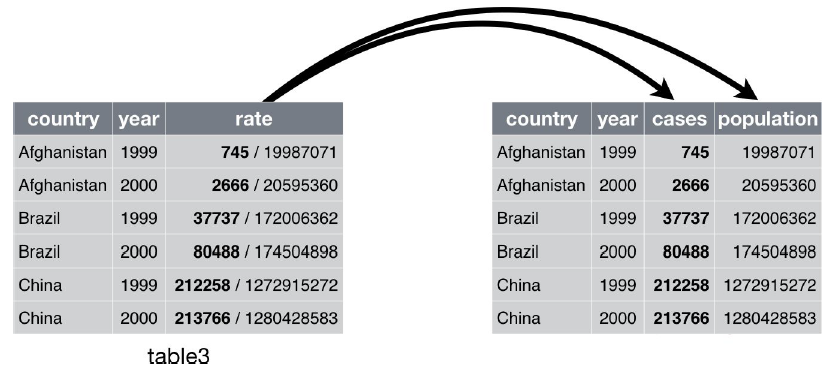
By default, separate() will split values wherever it sees a nonalphanumeric character (i.e., a character that isn’t a number or letter).
table3 %>%
separate(rate, into=c("cases","population"), sep="/")
## # A tibble: 6 × 4
## country year cases population
## <chr> <int> <chr> <chr>
## 1 Afghanistan 1999 745 19987071
## 2 Afghanistan 2000 2666 20595360
## 3 Brazil 1999 37737 172006362
## 4 Brazil 2000 80488 174504898
## 5 China 1999 212258 1272915272
## 6 China 2000 213766 1280428583
Did you find the problem/s?
## # A tibble: 6 × 4
## country year cases population
## <chr> <int> <chr> <chr>
## 1 Afghanistan 1999 745 19987071
## 2 Afghanistan 2000 2666 20595360
## 3 Brazil 1999 37737 172006362
## 4 Brazil 2000 80488 174504898
## 5 China 1999 212258 1272915272
## 6 China 2000 213766 1280428583
Convert the separated columns into correct data type
We can ask separate() to try and convert to better types using convert = TRUE:
table3 %>%
separate(
rate,
into = c("cases", "population"),
convert = TRUE
)
## # A tibble: 6 × 4
## country year cases population
## <chr> <int> <int> <int>
## 1 Afghanistan 1999 745 19987071
## 2 Afghanistan 2000 2666 20595360
## 3 Brazil 1999 37737 172006362
## 4 Brazil 2000 80488 174504898
## 5 China 1999 212258 1272915272
## 6 China 2000 213766 1280428583
Unite
unite() is the inverse of separate(): it combines multiple columns into a single column.
table5
## # A tibble: 6 × 4
## country century year rate
## * <chr> <chr> <chr> <chr>
## 1 Afghanistan 19 99 745/19987071
## 2 Afghanistan 20 00 2666/20595360
## 3 Brazil 19 99 37737/172006362
## 4 Brazil 20 00 80488/174504898
## 5 China 19 99 212258/1272915272
## 6 China 20 00 213766/1280428583
table5 %>%
unite(new, century, year)
## # A tibble: 6 × 3
## country new rate
## <chr> <chr> <chr>
## 1 Afghanistan 19_99 745/19987071
## 2 Afghanistan 20_00 2666/20595360
## 3 Brazil 19_99 37737/172006362
## 4 Brazil 20_00 80488/174504898
## 5 China 19_99 212258/1272915272
## 6 China 20_00 213766/1280428583
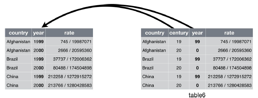
The default will place an underscore (_) between the values from different columns. Here we don’t want any separator so we use "":
table5 %>%
unite(new, century, year, sep="")
## # A tibble: 6 × 3
## country new rate
## <chr> <chr> <chr>
## 1 Afghanistan 1999 745/19987071
## 2 Afghanistan 2000 2666/20595360
## 3 Brazil 1999 37737/172006362
## 4 Brazil 2000 80488/174504898
## 5 China 1999 212258/1272915272
## 6 China 2000 213766/1280428583
Exercise
- Selecting year, month, flight, and tailnum columns from nycflights13::flights dataset.
- Combining year, and month with separator / in a new column, date.
- Then count the number of oberservations for each date, and sort by desc
Solution:
# use count() or group_by() with summarise() to # count the number of oberservations for each `date` flights %>% select(year, month, flight, tailnum) %>% unite(date, year, month, sep="/") %>% count(date, sort=T)
References
[1] Hadley Wickham, Garrett Grolemund. R For Data Science.
Data Wrangling with stringr, forcats (optional)
Data Wrangling with stringr and forcats [slides/code]
Environment
- R language
- R studio
Installation
install.pacages("tidyverse")
Visualizing Relational Data
introduction
It’s rare that a data analysis involves only a single table of data. Typically you have many tables of data, and you must combine them to answer the questions that you’re interested in. Collectively, multiple tables of data are called relational data because it is the relations, not just the individual datasets, that are important.
To work with relational data you need verbs that work with pairs of tables. There are two most common families of verbs designed to work with relational data:
-
Mutating joins, which add new variables to one data frame from matching observations in another.
-
Filtering joins, which filter observations from one data frame based on whether or not they match an observation in the other table.
Prerequisites
library(tidyverse)
library(nycflights13)
nycflights13
airlines lets you look up the full carrier name from its abbreviated code:
head(airlines)
## # A tibble: 6 × 2
## carrier name
## <chr> <chr>
## 1 9E Endeavor Air Inc.
## 2 AA American Airlines Inc.
## 3 AS Alaska Airlines Inc.
## 4 B6 JetBlue Airways
## 5 DL Delta Air Lines Inc.
## 6 EV ExpressJet Airlines Inc.
airports gives information about each airport, identified by the faa airport code:
airports
## # A tibble: 1,458 × 8
## faa name lat lon alt tz dst tzone
## <chr> <chr> <dbl> <dbl> <dbl> <dbl> <chr> <chr>
## 1 04G Lansdowne Airport 41.1 -80.6 1044 -5 A America/…
## 2 06A Moton Field Municipal Airport 32.5 -85.7 264 -6 A America/…
## 3 06C Schaumburg Regional 42.0 -88.1 801 -6 A America/…
## 4 06N Randall Airport 41.4 -74.4 523 -5 A America/…
## 5 09J Jekyll Island Airport 31.1 -81.4 11 -5 A America/…
## 6 0A9 Elizabethton Municipal Airport 36.4 -82.2 1593 -5 A America/…
## 7 0G6 Williams County Airport 41.5 -84.5 730 -5 A America/…
## 8 0G7 Finger Lakes Regional Airport 42.9 -76.8 492 -5 A America/…
## 9 0P2 Shoestring Aviation Airfield 39.8 -76.6 1000 -5 U America/…
## 10 0S9 Jefferson County Intl 48.1 -123. 108 -8 A America/…
## # … with 1,448 more rows
planes gives information about each plane, identified by its tailnum:
planes
## # A tibble: 3,322 × 9
## tailnum year type manufacturer model engines seats speed engine
## <chr> <int> <chr> <chr> <chr> <int> <int> <int> <chr>
## 1 N10156 2004 Fixed wing multi… EMBRAER EMB-… 2 55 NA Turbo…
## 2 N102UW 1998 Fixed wing multi… AIRBUS INDU… A320… 2 182 NA Turbo…
## 3 N103US 1999 Fixed wing multi… AIRBUS INDU… A320… 2 182 NA Turbo…
## 4 N104UW 1999 Fixed wing multi… AIRBUS INDU… A320… 2 182 NA Turbo…
## 5 N10575 2002 Fixed wing multi… EMBRAER EMB-… 2 55 NA Turbo…
## 6 N105UW 1999 Fixed wing multi… AIRBUS INDU… A320… 2 182 NA Turbo…
## 7 N107US 1999 Fixed wing multi… AIRBUS INDU… A320… 2 182 NA Turbo…
## 8 N108UW 1999 Fixed wing multi… AIRBUS INDU… A320… 2 182 NA Turbo…
## 9 N109UW 1999 Fixed wing multi… AIRBUS INDU… A320… 2 182 NA Turbo…
## 10 N110UW 1999 Fixed wing multi… AIRBUS INDU… A320… 2 182 NA Turbo…
## # … with 3,312 more rows
weather gives the weather at each NYC airport for each hour:
weather
## # A tibble: 26,115 × 15
## origin year month day hour temp dewp humid wind_dir wind_speed
## <chr> <int> <int> <int> <int> <dbl> <dbl> <dbl> <dbl> <dbl>
## 1 EWR 2013 1 1 1 39.0 26.1 59.4 270 10.4
## 2 EWR 2013 1 1 2 39.0 27.0 61.6 250 8.06
## 3 EWR 2013 1 1 3 39.0 28.0 64.4 240 11.5
## 4 EWR 2013 1 1 4 39.9 28.0 62.2 250 12.7
## 5 EWR 2013 1 1 5 39.0 28.0 64.4 260 12.7
## 6 EWR 2013 1 1 6 37.9 28.0 67.2 240 11.5
## 7 EWR 2013 1 1 7 39.0 28.0 64.4 240 15.0
## 8 EWR 2013 1 1 8 39.9 28.0 62.2 250 10.4
## 9 EWR 2013 1 1 9 39.9 28.0 62.2 260 15.0
## 10 EWR 2013 1 1 10 41 28.0 59.6 260 13.8
## # … with 26,105 more rows, and 5 more variables: wind_gust <dbl>, precip <dbl>,
## # pressure <dbl>, visib <dbl>, time_hour <dttm>
nycflights13 Entity Relationship Diagram
One way to show the relationships between the different tables is with a drawing: If you have taken database management, you would be familiar with.
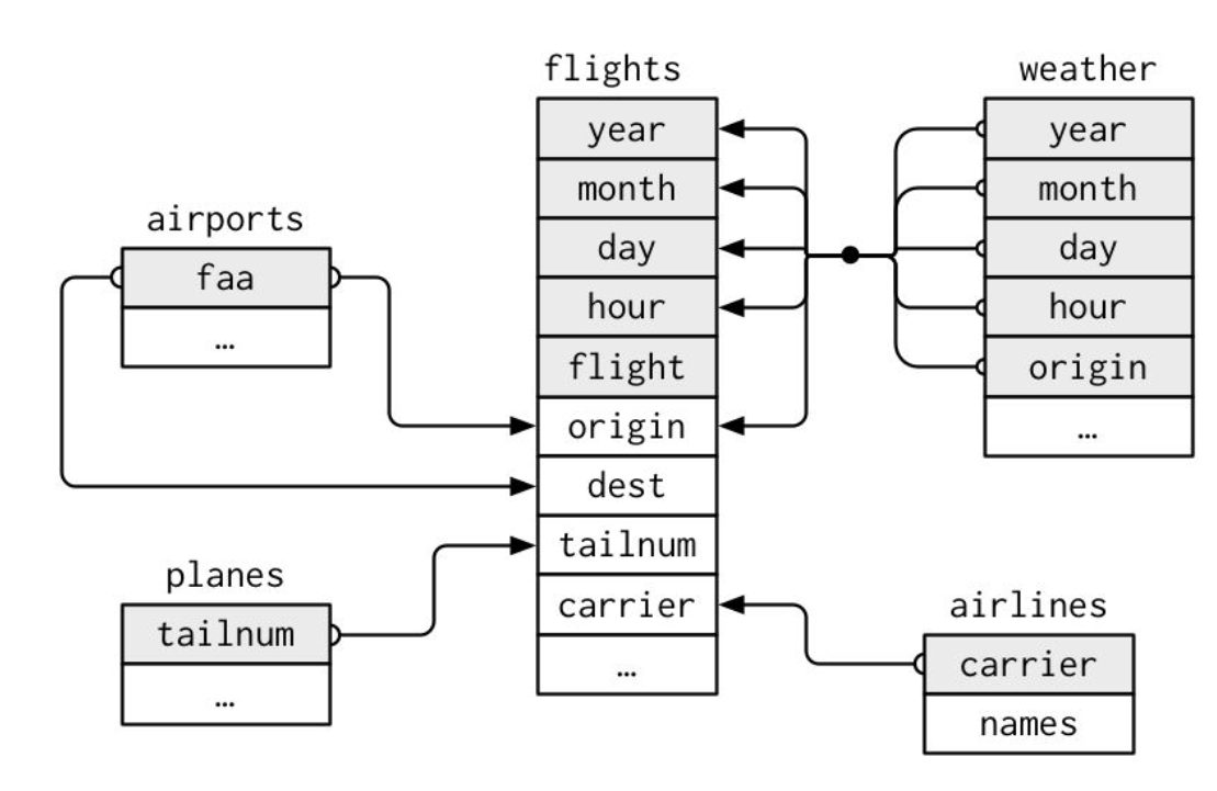
For nycflights13:
-
flights connects to planes via a single variable, tailnum.
-
flights connects to airlines through the carrier variable.
-
flights connects to airports in two ways: via the origin and dest variables.
-
flights connects to weather via origin (the location), and year, month, day, and hour (the time).
Key for relational data table
There are two types of keys:
-
A primary key uniquely identifies an observation in its own table.
-
A foreign key uniquely identifies an observation in another table.
Primary key (PK)
For example, planes$tailnum is a primary key because it uniquely identifies each plane in the planes table.
planes
## # A tibble: 3,322 × 9
## tailnum year type manufacturer model engines seats speed engine
## <chr> <int> <chr> <chr> <chr> <int> <int> <int> <chr>
## 1 N10156 2004 Fixed wing multi… EMBRAER EMB-… 2 55 NA Turbo…
## 2 N102UW 1998 Fixed wing multi… AIRBUS INDU… A320… 2 182 NA Turbo…
## 3 N103US 1999 Fixed wing multi… AIRBUS INDU… A320… 2 182 NA Turbo…
## 4 N104UW 1999 Fixed wing multi… AIRBUS INDU… A320… 2 182 NA Turbo…
## 5 N10575 2002 Fixed wing multi… EMBRAER EMB-… 2 55 NA Turbo…
## 6 N105UW 1999 Fixed wing multi… AIRBUS INDU… A320… 2 182 NA Turbo…
## 7 N107US 1999 Fixed wing multi… AIRBUS INDU… A320… 2 182 NA Turbo…
## 8 N108UW 1999 Fixed wing multi… AIRBUS INDU… A320… 2 182 NA Turbo…
## 9 N109UW 1999 Fixed wing multi… AIRBUS INDU… A320… 2 182 NA Turbo…
## 10 N110UW 1999 Fixed wing multi… AIRBUS INDU… A320… 2 182 NA Turbo…
## # … with 3,312 more rows
If we would likt to find one plane with tailnumber "N110UW"
planes %>%
filter(tailnum=="N110UW")
## # A tibble: 1 × 9
## tailnum year type manufacturer model engines seats speed engine
## <chr> <int> <chr> <chr> <chr> <int> <int> <int> <chr>
## 1 N110UW 1999 Fixed wing multi … AIRBUS INDU… A320… 2 182 NA Turbo…
Of course, the PK can be a combination of variables:c(year, month, day, hour, minute, origin)
flights %>%
filter(year==2013, month==1, day==5, hour==5, minute==40, origin=="JFK")
## # A tibble: 1 × 19
## year month day dep_time sched_dep_time dep_delay arr_time sched_arr_time
## <int> <int> <int> <int> <int> <dbl> <int> <int>
## 1 2013 1 5 537 540 -3 831 850
## # … with 11 more variables: arr_delay <dbl>, carrier <chr>, flight <int>,
## # tailnum <chr>, origin <chr>, dest <chr>, air_time <dbl>, distance <dbl>,
## # hour <dbl>, minute <dbl>, time_hour <dttm>
Foreign key
For example, flights$tailnum is a foreign key because it appears in the flights table where it matches each flight to a unique plane in the plane talbe. Which means in the table flights, the tailnum is a foreign key not a PK; but in the table plane, the tailnum is a PK
flights %>%
filter(tailnum=="N110UW")
## # A tibble: 40 × 19
## year month day dep_time sched_dep_time dep_delay arr_time sched_arr_time
## <int> <int> <int> <int> <int> <dbl> <int> <int>
## 1 2013 1 10 620 630 -10 855 831
## 2 2013 10 6 959 959 0 1214 1207
## 3 2013 10 9 1639 1540 59 1830 1742
## 4 2013 10 24 1600 1550 10 1756 1752
## 5 2013 11 6 1546 1544 2 1741 1750
## 6 2013 11 9 1458 1500 -2 1649 1656
## 7 2013 11 10 818 825 -7 1007 1029
## 8 2013 11 13 1540 1544 -4 1738 1750
## 9 2013 11 21 1222 1200 22 1413 1359
## 10 2013 11 26 1603 1544 19 1842 1750
...
Mutate Join
Data table
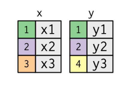
x <- tribble(
~key, ~val_x,
1, "x1",
2, "x2",
3, "x3"
)
y <- tribble(
~key, ~val_y,
1, "y1",
2, "y2",
4, "y3"
)
Inner join
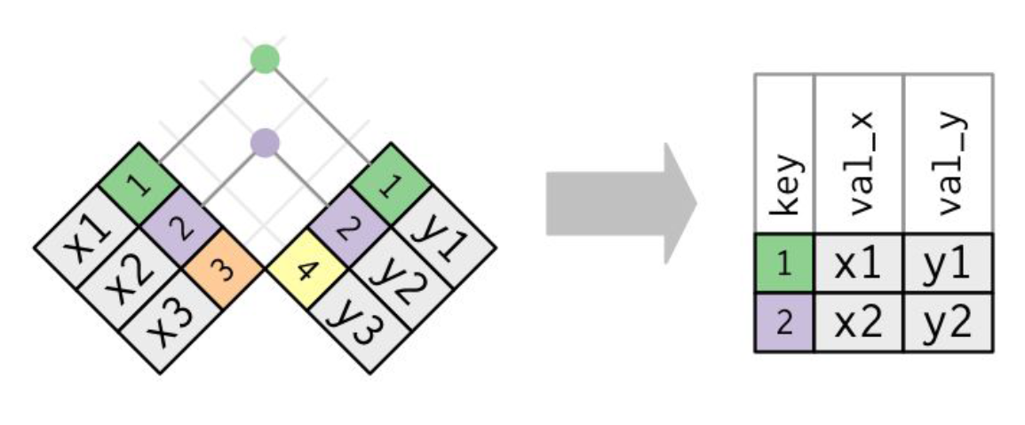
Base R functoin:
merge(x, y, by="key")
#or
x %>%
merge(y, by="key")
dplyr inner_join() function:
inner_join(x, y, by="key")
## # A tibble: 2 × 3
## key val_x val_y
## <dbl> <chr> <chr>
## 1 1 x1 y1
## 2 2 x2 y2
#or
x %>%
inner_join(y, by="key")
## # A tibble: 2 × 3
## key val_x val_y
## <dbl> <chr> <chr>
## 1 1 x1 y1
## 2 2 x2 y2
If the keys are different
Data
x <- tribble(
~key, ~val_x,
1, "x1",
2, "x2",
3, "x3"
)
y1 <- tribble(
~key1, ~val_y,
1, "y1",
2, "y2",
4, "y3"
)
Base function:
merge(x, y1, by.x="key", by.y="key1")
dplyr function:
inner_join(x, y1, by=c("key"="key1"))
Left join
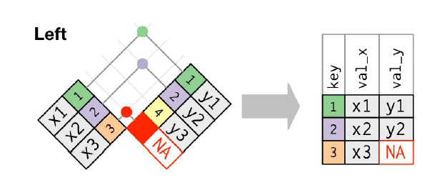
Base R functoin:
merge(x, y, by="key", all.x=TRUE)
#or
x %>%
merge(y, by="key", all.x=TRUE)
dplyr left_join() function:
left_join(x, y, by="key")
## # A tibble: 3 × 3
## key val_x val_y
## <dbl> <chr> <chr>
## 1 1 x1 y1
## 2 2 x2 y2
## 3 3 x3 <NA>
#or
x %>%
left_join(y, by="key")
## # A tibble: 3 × 3
## key val_x val_y
## <dbl> <chr> <chr>
## 1 1 x1 y1
## 2 2 x2 y2
## 3 3 x3 <NA>
Right join
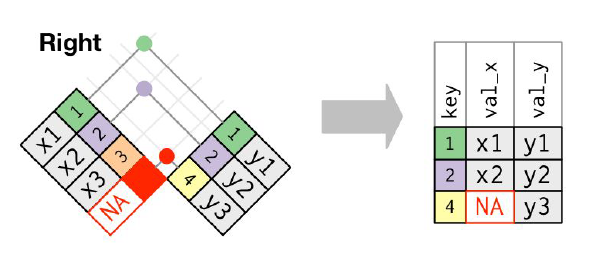
Base R functoin:
merge(x, y, by="key", all.y=TRUE)
#or
x %>%
merge(y, by="key", all.y=TRUE)
dplyr right_join() function:
right_join(x, y, by="key")
## # A tibble: 3 × 3
## key val_x val_y
## <dbl> <chr> <chr>
## 1 1 x1 y1
## 2 2 x2 y2
## 3 4 <NA> y3
#or
x %>%
right_join(y, by="key")
## # A tibble: 3 × 3
## key val_x val_y
## <dbl> <chr> <chr>
## 1 1 x1 y1
## 2 2 x2 y2
## 3 4 <NA> y3
Full join
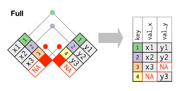
Base R functoin:
merge(x, y, by="key",
all.x=TRUE,
all.y = TRUE)
#or
x %>%
merge(y, by="key",
all.x=TRUE,
all.y = TRUE)
dplyr full_join() function:
full_join(x, y, by="key")
## # A tibble: 4 × 3
## key val_x val_y
## <dbl> <chr> <chr>
## 1 1 x1 y1
## 2 2 x2 y2
## 3 3 x3 <NA>
## 4 4 <NA> y3
#or
x %>%
full_join(y, by="key")
## # A tibble: 4 × 3
## key val_x val_y
## <dbl> <chr> <chr>
## 1 1 x1 y1
## 2 2 x2 y2
## 3 3 x3 <NA>
## 4 4 <NA> y3
Filtering Joins
- semi_join(x, y) keeps all observations in x that have a match in y.
- anti_join(x, y) drops all observations in x that have a match in y.
Semi-join
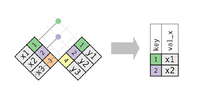
semi_join(x, y) keeps all observations in x that have a match in y.
Anti-join
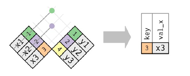
anti_join(x, y) drops all observations in x that have a match in y.
References
[1] Hadley Wickham, Garrett Grolemund. R For Data Science.
Introduction to Shiny
R shiny Topics
- Introduction to
shinyinteractive visualization web app [slides] shinyreactive output [slides/code]
Environment
- R language
- R studio
Installation of shiny
install.pacages("shiny")
Exploratory Data Analysis and More Data Visualization
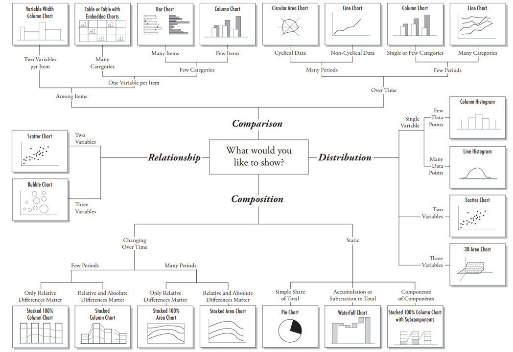
Materials
EDA and Advanced Visualization [slides/code]
EDA Topics
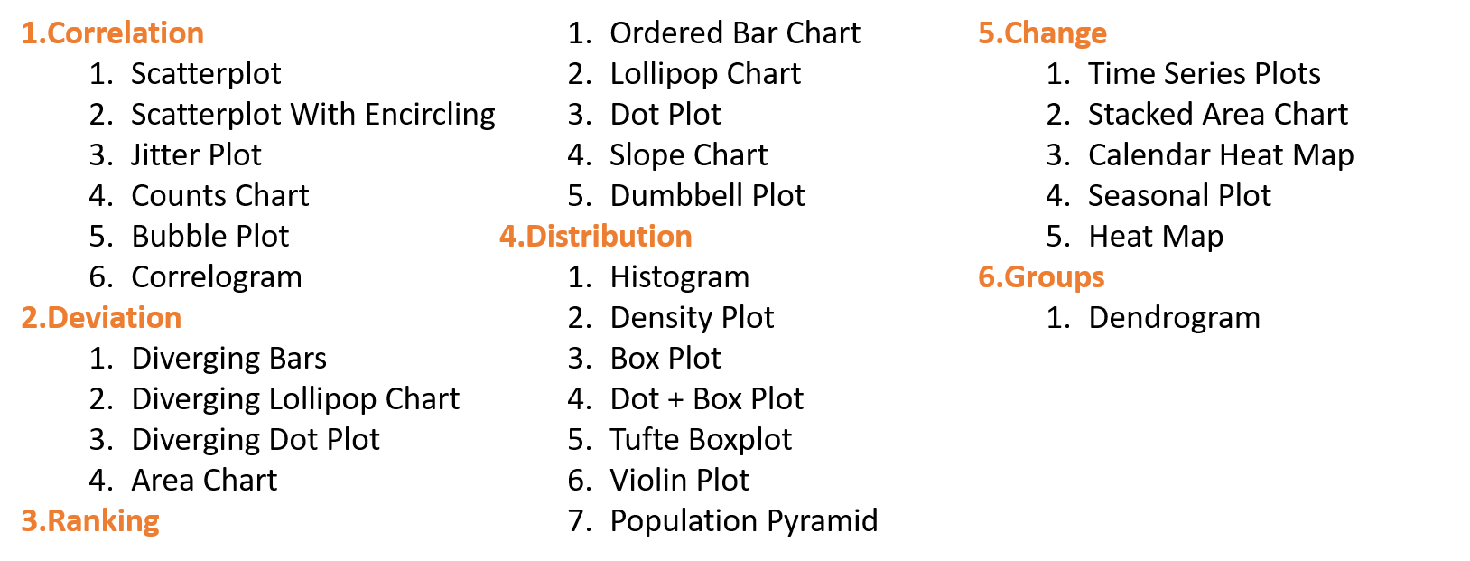
Advanced Visualization Topics
- Visualization by PCA
- Spatial Visualization
- Network Visualization
- Animated Visualization
- Interactive Visualization
- Polishing Procedure
R Modeling Workshop
R Modeling Workshop. [Github (included the slides and R code):]

Workshop Topics
The purpose of the workshop is to make students familiar with how to implement machine learning models by using R.
- Introduction to neural network and deep learning
- Principle Components Analysis (PCA) for Visualization
- k nearest neighbours (KNN) (Optional)
- Logistic Regression
Environment
- R language
- R studio
Installation of Keras and Tensorflow in R
The Keras R interface uses the TensorFlow backend engine by default.
install.packages("keras")
or install the development version with:
devtools::install_github("rstudio/keras")
then
library(keras)
install_keras()
@book{lu2022visualization,
title = "Data Visualization Tutorial in R",
author = "Lu, Zhenyuan",
year = "2022",
publisher = "zhenyuanlu.github.io",
url = "https://zhenyuanlu.com/r-comput-viz/"
}

